By: Picaud Vincent
Re-posted from: https://pixorblog.wordpress.com/2018/02/23/julia-dispatch-enum-vs-type-comparison/
Table of Contents
1 Context
Imagine the following scenario: a function func must efficiently calls a (short) subroutine belonging to predefined set of specialized functions. The chosen specialization is done thanks to a tag argument. Something like:
specialization(x,tag_1) = specialization 1
specialization(x,tag_2) = specialization 2
etc.

function func(tag)
  # some code
  for i in range
     specialization(x,tag)
  end
  # some code
end
Like specialization is called often, an efficient solution to perform the dispatching is desired.
Here I check two Julia solutions, one using @enum, the other using Type.
2 @enum based approach
Coming from the C++ world, I will start from the following C++ code to propose a Julia solution:
#include <iostream>
#include <type_traits>

enum Tags { A, B, C }; // I do not used enum class on purpose,
                       // to have A,B,C... as global identifiers

auto specialized(int x, std::integral_constant<Tags, A>)
{ return 1 * x; }
auto specialized(int x, std::integral_constant<Tags, B>)
{ return 2 * x; }
auto specialized(int x, std::integral_constant<Tags, C>)
{ return 3 * x; }

template <Tags TAG>
constexpr auto Tags_v = std::integral_constant<Tags,TAG>();

template <Tags TAG>
auto func(std::integral_constant<Tags, TAG> tag)
{
  return specialized(10, tag); // no run-time penalty
}

int main()
{
  std::cout << func(Tags_v<B>);
}
In C++, there is no run-time penalty because the right specialization is chosen at compile-time. In basic situations like this one, the compiler even inline everything.
Julia provides an @enum macro. To mimic the C++ std::integral_constant we use the Type{Val{.}} trick.
@enum Tags A B C

specialized(x::Int,::Type{Val{A}}) = 1*x
specialized(x::Int,::Type{Val{B}}) = 2*x
specialized(x::Int,::Type{Val{C}}) = 3*x

func(::Type{Val{e}}) where {e} = specialized(10,Val{e})
This work as exepected:
func(Val{B})
20
The generated assembly code confirms that everything is inlined as in C++.
@code_native func(Val{B})
	.text
Filename: none
	pushq	%rbp
	movq	%rsp, %rbp
Source line: 1
	movl	$20, %eax
	popq	%rbp
	retq
	nopl	(%rax,%rax)
Comparison with C++:
The C++ code is 13 lines long whereas the Julia one is only 5 lines long. The call site syntax is nearly the same:
func(Tags_v<A>);
versus
func(Val{B})
However, concerning the Julia solution, I have a minor regret. AFAIK in Julia we can not filter argument e with something like
func(::Type{Val{e}}) where {e::Tags} = specialized(10,Val{e}) # illegal code
This has several disadvantages. The code is less readable, not clearly showing our intent and argument restriction. Also, in case of bad use of the function, the error message is delayed until no specialization is found. For instance you can write:
func(Val{1})
and you will get the following error message:
julia> ERROR: MethodError: no method matching specialized(::Int64, ::Type{Val{1}})
Closest candidates are:
  specialized(::Int64, !Matched::Type{Val{A::Tags = 0}}) at none:1
  specialized(::Int64, !Matched::Type{Val{B::Tags = 1}}) at none:1
  specialized(::Int64, !Matched::Type{Val{C::Tags = 2}}) at none:1
Stacktrace:
 [1] func(::Type{Val{1}}) at ./none:1
The problem is that you have to search through the Stacktrace to find the origin of the error. In this simple example the answer is immediate but for deeper stracktrace maybe this can be the source of painful debugging.
In comparison, a compilation attempt of this C++ code:
func(Tags_v<1>)
prints an error message pointing directly at the call site:
test.cpp:22:21: error: invalid conversion from ‘int’ to ‘Tags’ [-fpermissive]
   func(Tags_v<1>);
               ^~~~~~~~~
3 Type based solution
In C++ a possible implementation is:
#include <iostream>
#include <type_traits>

struct Tags {};
struct A : Tags {};
struct B : Tags {};
struct C : Tags {};

auto specialized(int x, A) { return 1 * x; }
auto specialized(int x, B) { return 2 * x; }
auto specialized(int x, C) { return 3 * x; }

template <typename TAG,typename ENABLED = std::enable_if_t<std::is_base_of<Tags,TAG>::value>>
auto func(TAG tag)
{
  return specialized(10, tag); // no run-time penalty
}

int main()
{
  std::cout << func(B());
}
A Julia equivalent can be:
abstract type Tags end

struct A <: Tags end
struct B <: Tags end
struct C <: Tags end

specialized(x::Int,::Type{A}) = 1*x
specialized(x::Int,::Type{B}) = 2*x
specialized(x::Int,::Type{C}) = 3*x

func(::Type{T}) where {T<:Tags} = specialized(10,T)

func(B)
A look at the generated assembly code also confirms that everything is inlined:
@code_native func(B)
	.text
Filename: none
	pushq	%rbp
	movq	%rsp, %rbp
Source line: 1
	movl	$20, %eax
	popq	%rbp
	retq
	nopl	(%rax,%rax)
Comparison with C++:
The Julia code is still shorter. The two syntax
func(B)
versus
func(B()); // (or func<A>() if we choose another implementation)
is in favor of Julia (as Julia directly supports DataType, no instantiation of B is required).
With the Type approach Julia does not suffer anymore from the “argument filtering” problem we had with the @enum approach.
For instance:
func(1)
prints the following error message:
  : ERROR: MethodError: no method matching func(::Int64)
  : Closest candidates are:
  :   func(!Matched::Type{T<:Tags}) where T<:Tags at none:1
which points directly to the call site.
4 Default value and keyword argument
4.1 Default value
In C++ or Julia we can modify the func function to support a default value:
In C++:
enumapproach
template <Tags TAG=Tags::A>
auto func(std::integral_constant<Tags, TAG> tag=Tags_v<A>)
{
  return specialized(10, tag);
}

std::cout << func()           // prints 10
std::cout << func(Tags_v<B>)  // prints 20
Typeapproach
template <typename TAG=A,typename ENABLED = std::enable_if_t<std::is_base_of_v<Tags,TAG>>>
auto func(TAG tag=A())
{
  return specialized(10, tag); // no run-time penalty
}

std::cout << func()     // prints 10
std::cout << func(B())  // prints 20
In Julia:
@enumapproach
func(::Type{Val{e}}=Val{A}) where {e} = specialized(10,Val{e})

func()       # prints 10
func(Val{B}) # prints 20
Typeapproach
func(::Type{T}=A) where {T<:Tags} = specialized(10,T)
func()  # prints 10
func(B) # prints 20
We can also check with @code_native that everything is inlined as before.
Comparison with C++:
Here there is a clear advantage in favor of Julia. In the C++ code you have to set the default value at two different places.
4.2 Keyword argument
There is no direct solution in C++. In Julia you can write:
@enumapproach
func_kwa(;tag::Type{Val{e}}=Val{A}) where {e} = specialized(10,Val{e})
Typeapproach
func_kwa(;tag::Type{T}=A) where {T<:Tags} = specialized(10,T)
However there is a bad surprise if you look at the generated code (my Julia version is v0.6):
@code_native func_kwa(tag=B)
The code is so long that I put it at the end of this post, a lot of work is done at run-time! In our context this is not an acceptable solution due to the induced performance penalty.
5 Conclusions
We have compared two solutions to select a specialized subroutine given a tag passed as function argument. One solution is based on @enum, the other one is based on Type.
For the considered basic example we have verified that there is not run-time penalty and that like in C++, Julia can inline the function.
IMHO the better solution seems to be one based on Type. The reason are twofold:
- better code readability,
- AFAIK with the
@enum/Type{Val{.}}approach, one can not filter argument directly at the call site.
We also have checked that:
- we can use default argument without run-time penalty,
- we can not use keyword argument because it seems that a lot of work is done at run-time (at least with my Julia version).
6 Annex: asm code for func_kwa(tag=B)
Julia version:
versioninfo()
  Julia Version 0.6.2
  Commit d386e40c17 (2017-12-13 18:08 UTC)
  Platform Info:
    OS: Linux (x86_64-pc-linux-gnu)
    CPU: Intel(R) Xeon(R) CPU E5-2603 v3 @ 1.60GHz
    WORD_SIZE: 64
    BLAS: libopenblas (USE64BITINT DYNAMIC_ARCH NO_AFFINITY Haswell)
    LAPACK: libopenblas64_
    LIBM: libopenlibm
    LLVM: libLLVM-3.9.1 (ORCJIT, haswell)
Note: same conclusion with the @enum approach, func_kwa(tag=Val{B}).
@code_native func_kwa(tag=B)
	   .text
   Filename: <missing>
	   pushq	%rbp
	   movq	%rsp, %rbp
	   pushq	%r15
	   pushq	%r14
	   pushq	%r13
	   pushq	%r12
	   pushq	%rbx
	   subq	$120, %rsp
	   movq	%rdi, %r14
	   movabsq	$140389732029024, %r13  # imm = 0x7FAF081B9260
	   movq	%fs:0, %r15
	   addq	$-10888, %r15           # imm = 0xD578
	   leaq	-64(%rbp), %r12
	   xorps	%xmm0, %xmm0
	   movups	%xmm0, -64(%rbp)
	   movq	$0, -48(%rbp)
	   movups	%xmm0, -96(%rbp)
	   movups	%xmm0, -112(%rbp)
	   movups	%xmm0, -128(%rbp)
	   movups	%xmm0, -144(%rbp)
	   movq	$0, -80(%rbp)
	   movq	$26, -160(%rbp)
	   movq	(%r15), %rax
	   movq	%rax, -152(%rbp)
	   leaq	-160(%rbp), %rax
	   movq	%rax, (%r15)
	   movq	$0, -72(%rbp)
   Source line: 0
	   movq	$0, -120(%rbp)
	   movq	8(%r14), %rcx
	   sarq	%rcx
	   testq	%rcx, %rcx
	   jle	L271
	   movq	(%r14), %rdx
	   movq	24(%r14), %rsi
	   movl	$1, %eax
	   leaq	-24387768(%r13), %rdi
	   nopw	(%rax,%rax)
   L176:
	   leaq	-1(%rax), %rbx
	   cmpq	%rsi, %rbx
	   jae	L431
	   movq	-8(%rdx,%rax,8), %rbx
	   testq	%rbx, %rbx
	   je	L364
	   movq	%rbx, -144(%rbp)
	   movq	%rbx, -136(%rbp)
	   cmpq	%rdi, %rbx
	   jne	L465
	   cmpq	%rsi, %rax
	   jae	L379
	   movq	(%rdx,%rax,8), %rbx
	   testq	%rbx, %rbx
	   je	L416
	   movq	%rbx, -128(%rbp)
	   movq	%rbx, -120(%rbp)
	   addq	$2, %rax
	   decq	%rcx
	   jne	L176
	   movq	%rbx, -80(%rbp)
	   jmp	L286
   L271:
	   leaq	43425776(%r13), %rbx
	   movq	%rbx, -120(%rbp)
	   movq	%rbx, -80(%rbp)
   L286:
	   leaq	-22171552(%r13), %rax
	   movq	%rax, -64(%rbp)
	   movq	%rbx, -56(%rbp)
	   addq	$-22171848, %r13        # imm = 0xFEADAF38
	   movq	%r13, -48(%rbp)
	   movabsq	$jl_apply_generic, %rax
	   movl	$3, %esi
	   movq	%r12, %rdi
	   callq	*%rax
	   movq	%rax, -72(%rbp)
	   movq	(%rax), %rax
	   movq	-152(%rbp), %rcx
	   movq	%rcx, (%r15)
	   leaq	-40(%rbp), %rsp
	   popq	%rbx
	   popq	%r12
	   popq	%r13
	   popq	%r14
	   popq	%r15
	   popq	%rbp
	   retq
   L364:
	   movabsq	$jl_throw, %rax
	   movq	%r13, %rdi
	   callq	*%rax
   L379:
	   movq	%rsp, %rcx
	   leaq	-16(%rcx), %rsi
	   movq	%rsi, %rsp
	   incq	%rax
	   movq	%rax, -16(%rcx)
	   movabsq	$jl_bounds_error_ints, %rax
	   movl	$1, %edx
	   movq	%r14, %rdi
	   callq	*%rax
   L416:
	   movabsq	$jl_throw, %rax
	   movq	%r13, %rdi
	   callq	*%rax
   L431:
	   movq	%rsp, %rcx
	   leaq	-16(%rcx), %rsi
	   movq	%rsi, %rsp
	   movq	%rax, -16(%rcx)
	   movabsq	$jl_bounds_error_ints, %rax
	   movl	$1, %edx
	   movq	%r14, %rdi
	   callq	*%rax
   L465:
	   movabsq	$jl_gc_pool_alloc, %rax
	   movl	$1456, %esi             # imm = 0x5B0
	   movl	$32, %edx
	   movq	%r15, %rdi
	   callq	*%rax
	   movq	%rax, %rbx
	   leaq	-21540240(%r13), %rax
	   movq	%rax, -8(%rbx)
	   movq	%rbx, -112(%rbp)
	   xorps	%xmm0, %xmm0
	   movups	%xmm0, (%rbx)
	   movq	-648819312(%r13), %rax
	   movq	56(%rax), %rax
	   testq	%rax, %rax
	   jne	L545
	   movabsq	$jl_throw, %rax
	   movq	%r13, %rdi
	   callq	*%rax
   L545:
	   movq	%rax, -104(%rbp)
	   movq	%rax, -64(%rbp)
	   leaq	-25545896(%r13), %rax
	   movq	%rax, -56(%rbp)
	   movabsq	$jl_f_getfield, %rax
	   xorl	%edi, %edi
	   movl	$2, %edx
	   movq	%r12, %rsi
	   callq	*%rax
	   movq	%rax, -96(%rbp)
	   movq	%rax, (%rbx)
	   testq	%rax, %rax
	   je	L632
	   movq	-8(%rbx), %rcx
	   andl	$3, %ecx
	   cmpq	$3, %rcx
	   jne	L632
	   testb	$1, -8(%rax)
	   jne	L632
	   movabsq	$jl_gc_queue_root, %rax
	   movq	%rbx, %rdi
	   callq	*%rax
   L632:
	   movl	$1432, %esi             # imm = 0x598
	   movl	$16, %edx
	   movq	%r15, %rdi
	   movabsq	$jl_gc_pool_alloc, %rax
	   callq	*%rax
	   addq	$-647092848, %r13       # imm = 0xD96E2590
	   movq	%r13, -8(%rax)
	   movq	%rax, -88(%rbp)
	   movq	%r14, (%rax)
	   movq	%rax, 8(%rbx)
	   testq	%rax, %rax
	   je	L712
	   movq	-8(%rbx), %rax
	   andl	$3, %eax
	   cmpq	$3, %rax
	   jne	L712
	   movabsq	$jl_gc_queue_root, %rax
	   movq	%rbx, %rdi
	   callq	*%rax
   L712:
	   movq	$-1, 16(%rbx)
	   movabsq	$jl_throw, %rax
	   movq	%rbx, %rdi
	   callq	*%rax
	   nop
![\gamma[k]=\sum\limits_{i\in\Omega^\alpha}\alpha[i]\beta[k+\lambda i],\text{ with }\lambda\in\mathbb{Z}^*\text{\ \ \ \ \ \ \ \ \ \ \ \ (1)}](https://s0.wp.com/latex.php?latex=%5Cgamma%5Bk%5D%3D%5Csum%5Climits_%7Bi%5Cin%5COmega%5E%5Calpha%7D%5Calpha%5Bi%5D%5Cbeta%5Bk%2B%5Clambda+i%5D%2C%5Ctext%7B+with+%7D%5Clambda%5Cin%5Cmathbb%7BZ%7D%5E%2A%5Ctext%7B%5C+%5C+%5C+%5C+%5C+%5C+%5C+%5C+%5C+%5C+%5C+%5C+%281%29%7D+&bg=ffffff&%23038;fg=1a1a1a&%23038;s=0 "\gamma[k]=\sum\limits_{i\in\Omega^\alpha}\alpha[i]\beta[k+\lambda i],\text{ with }\lambda\in\mathbb{Z}^*\text{\ \ \ \ \ \ \ \ \ \ \ \ (1)}")
 .
.  has been introduced to define:
  convolution
 cross-correlation
 the stationary wavelet transform (the so called
 our vector domain (or support), for instance
![\alpha[i]](https://s0.wp.com/latex.php?latex=%5Calpha%5Bi%5D&bg=ffffff&%23038;fg=1a1a1a&%23038;s=0 "\alpha[i]") is defined for
is defined for

 the scaled domain
 and
and 
 the relative complement of
  with respect to the set
  defined by
 , it is sufficient to introduce the left and right parts (that can be empty)

 ,
,  defined on
  ,
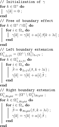
,  we want to define and implement an algorithm that computes
 ![\gamma[k]](https://s0.wp.com/latex.php?latex=%5Cgamma%5Bk%5D&bg=ffffff&%23038;fg=1a1a1a&%23038;s=0 "\gamma[k]") for
for  .
.  the domain that does not violate




![\gamma[k],\ k\in\Omega^\gamma](https://s0.wp.com/latex.php?latex=%5Cgamma%5Bk%5D%2C%5C+k%5Cin%5COmega%5E%5Cgamma&bg=ffffff&%23038;fg=1a1a1a&%23038;s=0 "\gamma[k],\ k\in\Omega^\gamma") (Eq. 1) is splitted into two parts:
(Eq. 1) is splitted into two parts:  free of boundary effect,
 that requires boundary extension
![\beta[.]](https://s0.wp.com/latex.php?latex=%5Cbeta%5B.%5D&bg=ffffff&%23038;fg=1a1a1a&%23038;s=0 "\beta[.]") and are sometimes entailed by a validity condition. For a better clarity I give explicit lower/upper bounds:
and are sometimes entailed by a validity condition. For a better clarity I give explicit lower/upper bounds: 


![\tilde{\beta}_j = \beta[2\,j_{min}-j]](https://s0.wp.com/latex.php?latex=%5Ctilde%7B%5Cbeta%7D_j++%3D+%5Cbeta%5B2%5C%2Cj_%7Bmin%7D-j%5D&bg=ffffff&%23038;fg=1a1a1a&%23038;s=0 "\tilde{\beta}_j = \beta[2\,j_{min}-j]")

![\tilde{\beta}_j = \beta[j_{max}-j_{min}+j+1]](https://s0.wp.com/latex.php?latex=%5Ctilde%7B%5Cbeta%7D_j+%3D++%5Cbeta%5Bj_%7Bmax%7D-j_%7Bmin%7D%2Bj%2B1%5D&bg=ffffff&%23038;fg=1a1a1a&%23038;s=0 "\tilde{\beta}_j = \beta[j_{max}-j_{min}+j+1]")

![\tilde{\beta}_j = \beta[j_{min}]](https://s0.wp.com/latex.php?latex=%5Ctilde%7B%5Cbeta%7D_j+%3D+%5Cbeta%5Bj_%7Bmin%7D%5D&bg=ffffff&%23038;fg=1a1a1a&%23038;s=0 "\tilde{\beta}_j = \beta[j_{min}]")



![\tilde{\beta}_j = \beta[2\,j_{max}-j]](https://s0.wp.com/latex.php?latex=%5Ctilde%7B%5Cbeta%7D_j++%3D+%5Cbeta%5B2%5C%2Cj_%7Bmax%7D-j%5D&bg=ffffff&%23038;fg=1a1a1a&%23038;s=0 "\tilde{\beta}_j = \beta[2\,j_{max}-j]")

![\tilde{\beta}_j = \beta[-j_{max}+j_{min}+j-1]](https://s0.wp.com/latex.php?latex=%5Ctilde%7B%5Cbeta%7D_j+%3D+%5Cbeta%5B-j_%7Bmax%7D%2Bj_%7Bmin%7D%2Bj-1%5D&bg=ffffff&%23038;fg=1a1a1a&%23038;s=0 "\tilde{\beta}_j = \beta[-j_{max}+j_{min}+j-1]")

![\tilde{\beta}_j = \beta[j_{max}]](https://s0.wp.com/latex.php?latex=%5Ctilde%7B%5Cbeta%7D_j+%3D+%5Cbeta%5Bj_%7Bmax%7D%5D&bg=ffffff&%23038;fg=1a1a1a&%23038;s=0 "\tilde{\beta}_j = \beta[j_{max}]")
 we want to define a periodic function
  of period
  . This function must fulfills the
 ![\tilde{\beta}[j+T]=\tilde{\beta}[j]](https://s0.wp.com/latex.php?latex=%5Ctilde%7B%5Cbeta%7D%5Bj%2BT%5D%3D%5Ctilde%7B%5Cbeta%7D%5Bj%5D&bg=ffffff&%23038;fg=1a1a1a&%23038;s=0 "\tilde{\beta}[j+T]=\tilde{\beta}[j]") relation.
relation.  where
where
 is the modulus function associated to a
  , we first translate the indices



 using
using  with
with
![\tilde{\beta}[U-j]=\tilde{\beta}[U+j]](https://s0.wp.com/latex.php?latex=%5Ctilde%7B%5Cbeta%7D%5BU-j%5D%3D%5Ctilde%7B%5Cbeta%7D%5BU%2Bj%5D&bg=ffffff&%23038;fg=1a1a1a&%23038;s=0 "\tilde{\beta}[U-j]=\tilde{\beta}[U+j]") relation for
relation for  .
.  using
using  (attention
  and not
  , otherwise the component
  is duplicated!).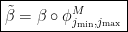


![\tilde{\beta}=\Phi(\beta,k+\lambda i)=\beta[\phi^X[k+\lambda i]]](https://s0.wp.com/latex.php?latex=%5Ctilde%7B%5Cbeta%7D%3D%5CPhi%28%5Cbeta%2Ck%2B%5Clambda+i%29%3D%5Cbeta%5B%5Cphi%5EX%5Bk%2B%5Clambda+i%5D%5D+&bg=ffffff&%23038;fg=1a1a1a&%23038;s=0 "\tilde{\beta}=\Phi(\beta,k+\lambda i)=\beta[\phi^X[k+\lambda i]]")
 is the boundary extension you have chosen (periodic, constant
 ). You do not have to take care of any validity condition, these formula are general.
  (access memory in the right order), use simd, or C++ meta-programming with loop unrolling for fixed
 in Julia, Fortran
 defined on
  (Julia) or
  (C++).
  .
. ![\alpha[i] = \tilde{\alpha}[\tilde{i}] = \tilde{\alpha}[i-l(\Omega^\alpha)+\tilde{i}_0]](https://s0.wp.com/latex.php?latex=%5Calpha%5Bi%5D+%3D++%5Ctilde%7B%5Calpha%7D%5B%5Ctilde%7Bi%7D%5D+%3D+%5Ctilde%7B%5Calpha%7D%5Bi-l%28%5COmega%5E%5Calpha%29%2B%5Ctilde%7Bi%7D_0%5D+&bg=ffffff&%23038;fg=1a1a1a&%23038;s=0 "\alpha[i] = \tilde{\alpha}[\tilde{i}] = \tilde{\alpha}[i-l(\Omega^\alpha)+\tilde{i}_0]")
![\gamma[k]=\sum\limits_{i\in\Omega^\alpha}\alpha[i]\beta[k+\lambda i] = \sum\limits_{i\in\Omega^\alpha}\tilde{\alpha}[i-l(\Omega^\alpha)+\tilde{i}_0]\beta[k+\lambda i]](https://s0.wp.com/latex.php?latex=%5Cgamma%5Bk%5D%3D%5Csum%5Climits_%7Bi%5Cin%5COmega%5E%5Calpha%7D%5Calpha%5Bi%5D%5Cbeta%5Bk%2B%5Clambda+i%5D+%3D+%5Csum%5Climits_%7Bi%5Cin%5COmega%5E%5Calpha%7D%5Ctilde%7B%5Calpha%7D%5Bi-l%28%5COmega%5E%5Calpha%29%2B%5Ctilde%7Bi%7D_0%5D%5Cbeta%5Bk%2B%5Clambda+i%5D+&bg=ffffff&%23038;fg=1a1a1a&%23038;s=0 "\gamma[k]=\sum\limits_{i\in\Omega^\alpha}\alpha[i]\beta[k+\lambda i] = \sum\limits_{i\in\Omega^\alpha}\tilde{\alpha}[i-l(\Omega^\alpha)+\tilde{i}_0]\beta[k+\lambda i]")
 we have

![\boxed{ \gamma[k]=\sum\limits_{\tilde{i}=\tilde{i}_0}^{u(\Omega^\alpha)-l(\Omega^\alpha)+\tilde{i}_0}\tilde{\alpha}[\tilde{i}]\beta[k+ \lambda \tilde{i} + \lambda (l(\Omega^\alpha) - \tilde{i}_0)]}](https://s0.wp.com/latex.php?latex=%5Cboxed%7B+%5Cgamma%5Bk%5D%3D%5Csum%5Climits_%7B%5Ctilde%7Bi%7D%3D%5Ctilde%7Bi%7D_0%7D%5E%7Bu%28%5COmega%5E%5Calpha%29-l%28%5COmega%5E%5Calpha%29%2B%5Ctilde%7Bi%7D_0%7D%5Ctilde%7B%5Calpha%7D%5B%5Ctilde%7Bi%7D%5D%5Cbeta%5Bk%2B+%5Clambda+%5Ctilde%7Bi%7D+%2B+%5Clambda+%28l%28%5COmega%5E%5Calpha%29+-+%5Ctilde%7Bi%7D_0%29%5D%7D+&bg=ffffff&%23038;fg=1a1a1a&%23038;s=0 "\boxed{ \gamma[k]=\sum\limits_{\tilde{i}=\tilde{i}_0}^{u(\Omega^\alpha)-l(\Omega^\alpha)+\tilde{i}_0}\tilde{\alpha}[\tilde{i}]\beta[k+ \lambda \tilde{i} + \lambda (l(\Omega^\alpha) - \tilde{i}_0)]}")
 other arrays are less problematic:
  . This does not reduce the generality of the subroutine.
 which is the output array, as for
  , but we provide
  to define the components we want to compute. The other components,
  , will remain unmodified by the subroutine.

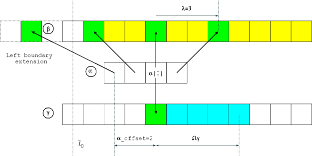
 you are in the “usual situation”. If you have a window size of
  , taking
  returns the middle of the window. Here, in the Fig. below, the graphical representation of an arbitrary case: a filter if size
  , with
  and
and  .
. 
 operator.

 arrays (not
  ones): some conjugation are missing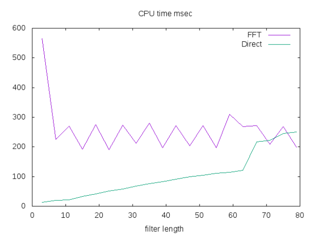
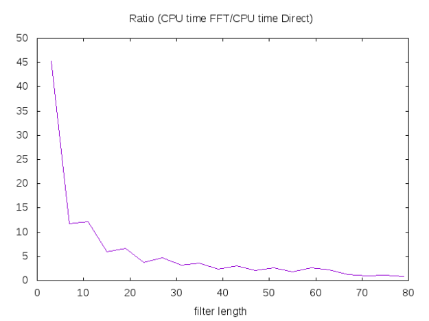
 domain
 .
. 

 domain
 what is the domain of


 with values

 in the middle of the window assuming that the
  are founded solving a least-squares problem:
 is our signal values and
  is the

 we get
 in a vector
  . Lets rewrite this in matrix form: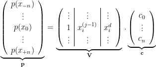


 where
where  is a diagonal matrix:

 we get:
 we get:
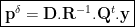
 .
.  points and a polynomial of degree
  we get: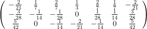
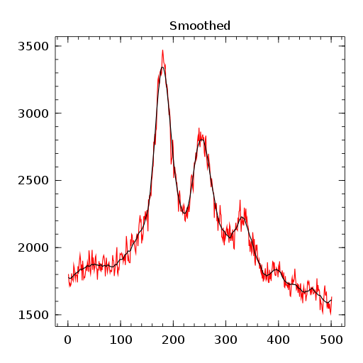
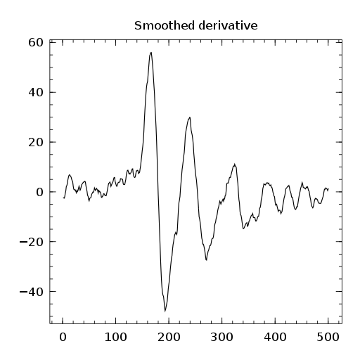
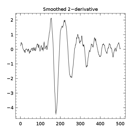
 filter, the second one the smoothed first order derivative
  filter and the last one the smoothed second order derivative
  filter.
 ![\gamma[k]=\sum\limits_i\alpha[i]\beta[k+\lambda i],\ with\ \lambda\in\mathbb{Z}^*](https://s0.wp.com/latex.php?latex=%5Cgamma%5Bk%5D%3D%5Csum%5Climits_i%5Calpha%5Bi%5D%5Cbeta%5Bk%2B%5Clambda+i%5D%2C%5C+with%5C+%5Clambda%5Cin%5Cmathbb%7BZ%7D%5E%2A+&bg=ffffff&%23038;fg=1a1a1a&%23038;s=0 "\gamma[k]=\sum\limits_i\alpha[i]\beta[k+\lambda i],\ with\ \lambda\in\mathbb{Z}^*")
 ,
,