By: Picaud Vincent
Re-posted from: https://pixorblog.wordpress.com/2016/07/17/direct-convolution/
For small kernels, direct convolution beats FFT based one. I present here a basic implementation. This implementation allows to compute
![\gamma[k]=\sum\limits_{i\in\Omega^\alpha}\alpha[i]\beta[k+\lambda i],\text{ with }\lambda\in\mathbb{Z}^*\text{\ \ \ \ \ \ \ \ \ \ \ \ (1)}](https://s0.wp.com/latex.php?latex=%5Cgamma%5Bk%5D%3D%5Csum%5Climits_%7Bi%5Cin%5COmega%5E%5Calpha%7D%5Calpha%5Bi%5D%5Cbeta%5Bk%2B%5Clambda+i%5D%2C%5Ctext%7B+with+%7D%5Clambda%5Cin%5Cmathbb%7BZ%7D%5E%2A%5Ctext%7B%5C+%5C+%5C+%5C+%5C+%5C+%5C+%5C+%5C+%5C+%5C+%5C+%281%29%7D+&bg=ffffff&%23038;fg=1a1a1a&%23038;s=0 "\gamma[k]=\sum\limits_{i\in\Omega^\alpha}\alpha[i]\beta[k+\lambda i],\text{ with }\lambda\in\mathbb{Z}^*\text{\ \ \ \ \ \ \ \ \ \ \ \ (1)}")
From time to time we will use the notation 
An arbitrary stride 
convolution
cross-correlation
the stationary wavelet transform (the so called “à trous” algorithm)
Also note that with proper boundary extension (periodic and zero padding essentially), changing the sign of

Disclaimer
Maybe the following is overwhelmingly detailed for a simple task like Eq. (1), but I have found some interests in writing this once for all. Maybe it can be useful for someone else.
Some notations
We note 

means that ![\alpha[i]](https://s0.wp.com/latex.php?latex=%5Calpha%5Bi%5D&bg=ffffff&%23038;fg=1a1a1a&%23038;s=0 "\alpha[i]")

To get interval lower/upper bounds we use the notation
\text{ and }i_{\max}=u(\Omega^\alpha)")
We denote by 

where }")
}")
Finally we use 


 \wedge (i\notin B) \}")
This set is not necessary connex, however like we are working in 
_{\text{Left}}=\llbracket l(A), \min{(u(A),l(B)-1)} \rrbracket")
_{\text{Right}}=\llbracket \max{(l(A),u(B)+1)}, u(A) \rrbracket")
Goal
Given two vectors 


![\gamma[k]](https://s0.wp.com/latex.php?latex=%5Cgamma%5Bk%5D&bg=ffffff&%23038;fg=1a1a1a&%23038;s=0 "\gamma[k]")

First step, no boundary extension
We need to define the 

Let’s write the details,
\Leftrightarrow (\forall i \in \Omega^\alpha \Rightarrow l(\Omega^\beta)-\lambda i \le k \le u(\Omega^\beta)-\lambda i)")
-\lambda i \le k \le \min\limits_{i\in \Omega^\alpha} u(\Omega^\beta)-\lambda i")
-l(\lambda \Omega^\alpha) \le k \le u(\Omega^\beta)-u(\lambda \Omega^\alpha)")
hence we have
-l(\lambda \Omega^\alpha) , u(\Omega^\beta)-u(\lambda \Omega^\alpha) \rrbracket }")
Thus the computation of ![\gamma[k],\ k\in\Omega^\gamma](https://s0.wp.com/latex.php?latex=%5Cgamma%5Bk%5D%2C%5C+k%5Cin%5COmega%5E%5Cgamma&bg=ffffff&%23038;fg=1a1a1a&%23038;s=0 "\gamma[k],\ k\in\Omega^\gamma")
- one part
free of boundary effect,
- one part
that requires boundary extension
")
The algorithm takes the following form:
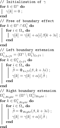
Second step, boundary extensions
Usually we define some classical boundary extensions. These extensions are computed from ![\beta[.]](https://s0.wp.com/latex.php?latex=%5Cbeta%5B.%5D&bg=ffffff&%23038;fg=1a1a1a&%23038;s=0 "\beta[.]")

Left boundary ") |
") |
validity condition |
|---|---|---|
| Mirror | ![\tilde{\beta}_j = \beta[2\,j_{min}-j]](https://s0.wp.com/latex.php?latex=%5Ctilde%7B%5Cbeta%7D_j++%3D+%5Cbeta%5B2%5C%2Cj_%7Bmin%7D-j%5D&bg=ffffff&%23038;fg=1a1a1a&%23038;s=0 "\tilde{\beta}_j = \beta[2\,j_{min}-j]") |
 |
| Periodic (or cyclic) | ![\tilde{\beta}_j = \beta[j_{max}-j_{min}+j+1]](https://s0.wp.com/latex.php?latex=%5Ctilde%7B%5Cbeta%7D_j+%3D++%5Cbeta%5Bj_%7Bmax%7D-j_%7Bmin%7D%2Bj%2B1%5D&bg=ffffff&%23038;fg=1a1a1a&%23038;s=0 "\tilde{\beta}_j = \beta[j_{max}-j_{min}+j+1]") |
 |
| Constant | ![\tilde{\beta}_j = \beta[j_{min}]](https://s0.wp.com/latex.php?latex=%5Ctilde%7B%5Cbeta%7D_j+%3D+%5Cbeta%5Bj_%7Bmin%7D%5D&bg=ffffff&%23038;fg=1a1a1a&%23038;s=0 "\tilde{\beta}_j = \beta[j_{min}]") |
none |
| Zero padding |  |
none |
Right boundary ") |
") |
validity condition |
|---|---|---|
| Mirror | ![\tilde{\beta}_j = \beta[2\,j_{max}-j]](https://s0.wp.com/latex.php?latex=%5Ctilde%7B%5Cbeta%7D_j++%3D+%5Cbeta%5B2%5C%2Cj_%7Bmax%7D-j%5D&bg=ffffff&%23038;fg=1a1a1a&%23038;s=0 "\tilde{\beta}_j = \beta[2\,j_{max}-j]") |
 |
| Periodic (or cyclic) | ![\tilde{\beta}_j = \beta[-j_{max}+j_{min}+j-1]](https://s0.wp.com/latex.php?latex=%5Ctilde%7B%5Cbeta%7D_j+%3D+%5Cbeta%5B-j_%7Bmax%7D%2Bj_%7Bmin%7D%2Bj-1%5D&bg=ffffff&%23038;fg=1a1a1a&%23038;s=0 "\tilde{\beta}_j = \beta[-j_{max}+j_{min}+j-1]") |
 |
| Constant | ![\tilde{\beta}_j = \beta[j_{max}]](https://s0.wp.com/latex.php?latex=%5Ctilde%7B%5Cbeta%7D_j+%3D+%5Cbeta%5Bj_%7Bmax%7D%5D&bg=ffffff&%23038;fg=1a1a1a&%23038;s=0 "\tilde{\beta}_j = \beta[j_{max}]") |
none |
| Zero padding | |
none |
As we want something general we want to get rid of these validity conditions.
Periodic case
Starting from a vector 


![\tilde{\beta}[j+T]=\tilde{\beta}[j]](https://s0.wp.com/latex.php?latex=%5Ctilde%7B%5Cbeta%7D%5Bj%2BT%5D%3D%5Ctilde%7B%5Cbeta%7D%5Bj%5D&bg=ffffff&%23038;fg=1a1a1a&%23038;s=0 "\tilde{\beta}[j+T]=\tilde{\beta}[j]")
We can do that by considering ")
=\bmod_F(j,U+1)")
and 
For a vector defined on an arbitrary domain 
=j-j_{\min}")
and then translate them back using }_{j_{\min}}=\tau_{-j_{\min}}")
Putting all together, we build a periodized vector

where
}_{j_{\min}} \circ \phi^P_{j_{\max}- j_{\min}} \circ \tau_{j_{\min}}")
}")
Mirror Symmetry case
Starting from a vector 

=U-|U-j|")
The resulting vector ![\tilde{\beta}[U-j]=\tilde{\beta}[U+j]](https://s0.wp.com/latex.php?latex=%5Ctilde%7B%5Cbeta%7D%5BU-j%5D%3D%5Ctilde%7B%5Cbeta%7D%5BU%2Bj%5D&bg=ffffff&%23038;fg=1a1a1a&%23038;s=0 "\tilde{\beta}[U-j]=\tilde{\beta}[U+j]")

To get a “global” definition we then periodize it on 


For an arbitrary domain

where
}_{j_{\min}} \circ \phi^M_{j_{\max}- j_{\min}} \circ \phi^P_{2(j_{\max}- j_{\min})-1} \circ \tau_{j_{\min}}")
)| }")
Boundary extensions
To use the algorithm with boundary extensions, you only have to define:
![\tilde{\beta}=\Phi(\beta,k+\lambda i)=\beta[\phi^X[k+\lambda i]]](https://s0.wp.com/latex.php?latex=%5Ctilde%7B%5Cbeta%7D%3D%5CPhi%28%5Cbeta%2Ck%2B%5Clambda+i%29%3D%5Cbeta%5B%5Cphi%5EX%5Bk%2B%5Clambda+i%5D%5D+&bg=ffffff&%23038;fg=1a1a1a&%23038;s=0 "\tilde{\beta}=\Phi(\beta,k+\lambda i)=\beta[\phi^X[k+\lambda i]]")
where 
 ). You do not have to take care of any validity condition, these formula are general.
Implementation
This is a straightforward implementation following as close as possible the presented formula. We did not try to optimize it, this would have obscured the presentation. Some ideas: reverse 

Preamble
Index translation / domain definition
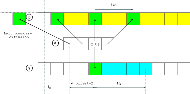
There is however one last thing we have to explain. In languages like Julia, C we are manipulating arrays having a common starting index:  or
or
For this reason we do not manipulate 


To cover all cases, I assume that the starting index is denoted by 
The array
![\alpha[i] = \tilde{\alpha}[\tilde{i}] = \tilde{\alpha}[i-l(\Omega^\alpha)+\tilde{i}_0]](https://s0.wp.com/latex.php?latex=%5Calpha%5Bi%5D+%3D++%5Ctilde%7B%5Calpha%7D%5B%5Ctilde%7Bi%7D%5D+%3D+%5Ctilde%7B%5Calpha%7D%5Bi-l%28%5COmega%5E%5Calpha%29%2B%5Ctilde%7Bi%7D_0%5D+&bg=ffffff&%23038;fg=1a1a1a&%23038;s=0 "\alpha[i] = \tilde{\alpha}[\tilde{i}] = \tilde{\alpha}[i-l(\Omega^\alpha)+\tilde{i}_0]")
Hence we must modify the initiale Eq. (1) to use
![\gamma[k]=\sum\limits_{i\in\Omega^\alpha}\alpha[i]\beta[k+\lambda i] = \sum\limits_{i\in\Omega^\alpha}\tilde{\alpha}[i-l(\Omega^\alpha)+\tilde{i}_0]\beta[k+\lambda i]](https://s0.wp.com/latex.php?latex=%5Cgamma%5Bk%5D%3D%5Csum%5Climits_%7Bi%5Cin%5COmega%5E%5Calpha%7D%5Calpha%5Bi%5D%5Cbeta%5Bk%2B%5Clambda+i%5D+%3D+%5Csum%5Climits_%7Bi%5Cin%5COmega%5E%5Calpha%7D%5Ctilde%7B%5Calpha%7D%5Bi-l%28%5COmega%5E%5Calpha%29%2B%5Ctilde%7Bi%7D_0%5D%5Cbeta%5Bk%2B%5Clambda+i%5D+&bg=ffffff&%23038;fg=1a1a1a&%23038;s=0 "\gamma[k]=\sum\limits_{i\in\Omega^\alpha}\alpha[i]\beta[k+\lambda i] = \sum\limits_{i\in\Omega^\alpha}\tilde{\alpha}[i-l(\Omega^\alpha)+\tilde{i}_0]\beta[k+\lambda i]")
With +\tilde{i}_0")
-l(\Omega^\alpha)+\tilde{i}_0 \rrbracket")
and
 - \tilde{i}_0)}_{\beta\_\text{offset}}")
Thus, Eq (1) becomes:
![\boxed{ \gamma[k]=\sum\limits_{\tilde{i}=\tilde{i}_0}^{u(\Omega^\alpha)-l(\Omega^\alpha)+\tilde{i}_0}\tilde{\alpha}[\tilde{i}]\beta[k+ \lambda \tilde{i} + \lambda (l(\Omega^\alpha) - \tilde{i}_0)]}](https://s0.wp.com/latex.php?latex=%5Cboxed%7B+%5Cgamma%5Bk%5D%3D%5Csum%5Climits_%7B%5Ctilde%7Bi%7D%3D%5Ctilde%7Bi%7D_0%7D%5E%7Bu%28%5COmega%5E%5Calpha%29-l%28%5COmega%5E%5Calpha%29%2B%5Ctilde%7Bi%7D_0%7D%5Ctilde%7B%5Calpha%7D%5B%5Ctilde%7Bi%7D%5D%5Cbeta%5Bk%2B+%5Clambda+%5Ctilde%7Bi%7D+%2B+%5Clambda+%28l%28%5COmega%5E%5Calpha%29+-+%5Ctilde%7Bi%7D_0%29%5D%7D+&bg=ffffff&%23038;fg=1a1a1a&%23038;s=0 "\boxed{ \gamma[k]=\sum\limits_{\tilde{i}=\tilde{i}_0}^{u(\Omega^\alpha)-l(\Omega^\alpha)+\tilde{i}_0}\tilde{\alpha}[\tilde{i}]\beta[k+ \lambda \tilde{i} + \lambda (l(\Omega^\alpha) - \tilde{i}_0)]}")
The 
- For
. This does not reduce the generality of the subroutine.
- For
which is the output array, as for
, but we provide
to define the components we want to compute. The other components,
, will remain unmodified by the subroutine.
Definition of 
As we have seen before, the convolution subroutine will have
 -1 \rrbracket")
Note: this definition does not depend on
With 


Julia
Auxiliary subroutines
We start by defining the basic operations on sets:
function scale(λ::Int64,Ω::UnitRange)
    ifelse(λ>0,
           UnitRange(λ*start(Ω),λ*last(Ω)),
           UnitRange(λ*last(Ω),λ*start(Ω)))
end

function compute_Ωγ1(Ωα::UnitRange,
                     λ::Int64,
                     Ωβ::UnitRange)

    λΩα = scale(λ,Ωα)

    UnitRange(start(Ωβ)-start(λΩα),
              last(Ωβ)-last(λΩα))
end

# Left & Right relative complements A\B
#
function relelativeComplement_left(A::UnitRange,
                                   B::UnitRange)
    UnitRange(start(A),
              min(last(A),start(B)-1))
end

function relelativeComplement_right(A::UnitRange,
                                    B::UnitRange)
    UnitRange(max(start(A),last(B)+1),
              last(A))
end
Boundary extensions
We then define the boundary extensions. Nothing special there, we only had to check that the Julia mod(x,y) function is the floored division version (by opposition to the rem(x,y) function which is the rounded toward zero division version).
const tilde_i0 = Int64(1)

function boundaryExtension_zeroPadding{T}(β::StridedVector{T},
                                          k::Int64)
    kmin = tilde_i0
    kmax = length(β) + kmin - 1

    if (k>=kmin)&&(k<=kmax)
        β[k]
    else
        T(0)
    end
end

function boundaryExtension_constant{T}(β::StridedVector{T},
                                       k::Int64)
    kmin = tilde_i0
    kmax = length(β) + kmin - 1

    if k<kmin
        β[kmin]
    elseif k<=kmax
        β[k]
    else
        β[kmax]
    end
end

function boundaryExtension_periodic{T}(β::StridedVector{T},
                                       k::Int64)
    kmin = tilde_i0
    kmax = length(β) + kmin - 1

    β[kmin+mod(k-kmin,1+kmax-kmin)]
end

function boundaryExtension_mirror{T}(β::StridedVector{T},
                                     k::Int64)
    kmin = tilde_i0
    kmax = length(β) + kmin - 1

    β[kmax-abs(kmax-kmin-mod(k-kmin,2*(kmax-kmin)))]
end

# For the user interface
#
boundaryExtension =
    Dict(:ZeroPadding=>boundaryExtension_zeroPadding,
         :Constant=>boundaryExtension_constant,
         :Periodic=>boundaryExtension_periodic,
         :Mirror=>boundaryExtension_mirror)
Main subroutine
Finally we define the main subroutine. Its arguments have been defined in the preamble part. I just added one @simd & @inbounds because this has a significant impact concerning perfomance (see end of this post).
function direct_conv!{T}(tilde_α::StridedVector{T},
                         Ωα::UnitRange,
                         λ::Int64,
                         β::StridedVector{T},
                         γ::StridedVector{T},
                         Ωγ::UnitRange,
                         LeftBoundary::Symbol,
                         RightBoundary::Symbol)
    # Sanity check
    @assert λ!=0
    @assert length(tilde_α)==length(Ωα)
    @assert (start(Ωγ)>=1)&&(last(Ωγ)<=length(γ))

    # Initialization
    Ωβ = UnitRange(1,length(β))
    tilde_Ωα = 1:length(Ωα)

    for k in Ωγ
        γ[k]=0
    end

    rΩγ1=intersect(Ωγ,compute_Ωγ1(Ωα,λ,Ωβ))

    # rΩγ1 part: no boundary effect
    #
    β_offset = λ*(start(Ωα)-tilde_i0)
    @simd for k in rΩγ1
        for i in tilde_Ωα
            @inbounds γ[k]+=tilde_α[i]*β[k+λ*i+β_offset]
        end
    end

    # Left part
    #
    rΩγ1_left = relelativeComplement_left(Ωγ,rΩγ1)
    Φ_left = boundaryExtension[LeftBoundary]

    for k in rΩγ1_left
        for i in tilde_Ωα
            γ[k]+=tilde_α[i]*Φ_left(β,k+λ*i+β_offset)
        end
    end

    # Right part
    #
    rΩγ1_right = relelativeComplement_right(Ωγ,rΩγ1)
    Φ_right = boundaryExtension[RightBoundary]

    for k in rΩγ1_right
        for i in tilde_Ωα
            γ[k]+=tilde_α[i]*Φ_right(β,k+λ*i+β_offset)
        end
    end
end

# Some UI functions, γ inplace modification
#
function direct_conv!{T}(tilde_α::StridedVector{T},
                         α_offset::Int64,
                         λ::Int64,

                         β::StridedVector{T},

                         γ::StridedVector{T},
                         Ωγ::UnitRange,

                         LeftBoundary::Symbol,
                         RightBoundary::Symbol)

    Ωα = UnitRange(-α_offset,
                   length(tilde_α)-α_offset-1)

    direct_conv!(tilde_α,
                 Ωα,
                 λ,

                 β,

                 γ,
                 Ωγ,

                 LeftBoundary,
                 RightBoundary)
end

# Some UI functions, allocates γ
#
function direct_conv{T}(tilde_α::StridedVector{T},
                        α_offset::Int64,
                        λ::Int64,

                        β::StridedVector{T},

                        LeftBoundary::Symbol,
                        RightBoundary::Symbol)

    γ = Array{T,1}(length(β))

    direct_conv!(tilde_α,
                 α_offset,
                 λ,

                 β,

                 γ,
                 UnitRange(1,length(γ)),

                 LeftBoundary,
                 RightBoundary)

    γ
end
In C/C++
As this post is already long I will not provide a complete code here. The only trap is to use the right mod function.
C/C++ modulus operator % is not standardized. Only the D%d=D-d*(D/d) relation is invariant allowing to define the Euclidean division. On the other side a lot of CPU x86 idiv, truncate toward zero, as a consequence C/C++ generally uses this direction.
To be sure, we have to explicitly use our F-mod function:
// Floored mod
int modF(int D, int d)
{
    int r = std::fmod(D,d);
    if((r > 0 && d < 0) || (r < 0 && d > 0)) r = r + d;
    return r;
}
You can read:
Usages examples
Basic usages
Beware that due to the asymmetric role of 
- Commutativity:

only for ZeroPadding
- Adjoint operator:

only for ZeroPadding and Periodic
- I have assumed
arrays (not
ones): some conjugation are missing
- Not considered here, but extension to n-dimensional & separable filters is immediate
push!(LOAD_PATH,"./")
using DirectConv

α=rand(4);
β=rand(10);

# Check adjoint operator
# -> restricted to ZeroPadding & Periodic
#    (asymmetric role of α and β)
#
vβ=rand(length(β))
d1=dot(direct_conv(α,2,-3,vβ,:ZeroPadding,:ZeroPadding),β)
d2=dot(direct_conv(α,2,+3,β,:ZeroPadding,:ZeroPadding),vβ)

@assert abs(d1-d2)<sqrt(eps())

d1=dot(direct_conv(α,-1,-3,vβ,:Periodic,:Periodic),β)
d2=dot(direct_conv(α,-1,+3,β,:Periodic,:Periodic),vβ)

@assert abs(d1-d2)<sqrt(eps())

# Check commutativity
# -> λ = -1 (convolution) and
#    restricted to ZeroPadding
#    (asymmetric role of α and β)
v1=zeros(20)
v2=zeros(20)
direct_conv!(α,0,-1,
             β,v1,UnitRange(1,20),:ZeroPadding,:ZeroPadding)
direct_conv!(β,0,-1,
             α,v2,UnitRange(1,20),:ZeroPadding,:ZeroPadding)

@assert (norm(v1-v2)<sqrt(eps()))

# Check Interval splitting
# (should work for any boundary extension type)
#
γ=direct_conv(α,3,2,β,:Mirror,:Periodic) # global computation
Γ=zeros(length(γ))
Ω1=UnitRange(1:3)
Ω2=UnitRange(4:length(γ))
direct_conv!(α,3,2,β,Γ,Ω1,:Mirror,:Periodic) # compute on Ω1
direct_conv!(α,3,2,β,Γ,Ω2,:Mirror,:Periodic) # compute on Ω2

@assert (norm(γ-Γ)<sqrt(eps()))
Performance?
In a previous post I gave a short derivation of the Savitzky-Golay filters. I used a FFT based convolution to apply the filters. It is interesting to compare the performance of the presented direct approach vs the FFT one.
push!(LOAD_PATH,"./")
using DirectConv

function apply_filter{T}(filter::StridedVector{T},signal::StridedVector{T})

    @assert isodd(length(filter))

    halfWindow = round(Int,(length(filter)-1)/2)

    padded_signal =
        [signal[1]*ones(halfWindow);
         signal;
         signal[end]*ones(halfWindow)]

    filter_cross_signal = conv(filter[end:-1:1],
                               padded_signal)

    filter_cross_signal[2*halfWindow+1:end-2*halfWindow]
end

# Now we can create a (very) rough benchmark
M=Array(Float64,0,3)
β=rand(1000000);
for halfWidth in 1:2:40
    α=rand(2*halfWidth+1);

    fft_t0 = time()
    fft_v = apply_filter(α,β)
    fft_t1 = time()

    direct_t0 = time()
    direct_v = direct_conv(α,halfWidth,1,β,
                           :Constant,:Constant)
    direct_t1 = time()

    @assert (norm(fft_v -direct_v)<sqrt(eps()))

    M=vcat(M,
           Float64[length(α)
                   (fft_t1-fft_t0)*1e3
                   (direct_t1-direct_t0)*1e3])
end
M
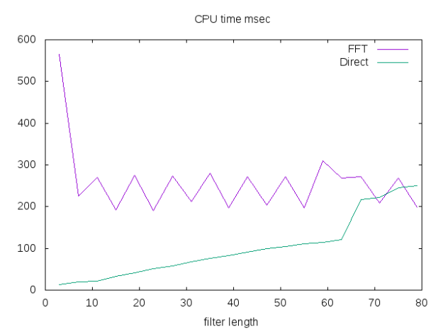
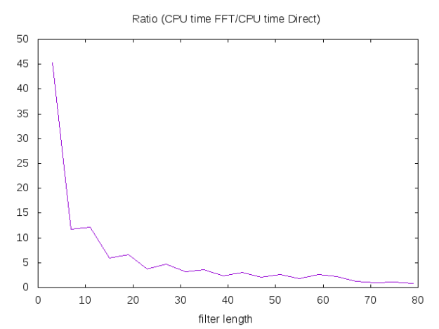
We see that for small filters direct method can easily be 10 time faster than the FFT approach!
Conclusion: for small filters, use a direct approach!
Discussion
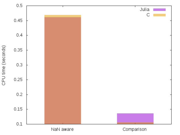
Optimization/performance
If I have time I will try to benchmark two basic implementations, a Julia one vs a C/C++ one. I’m a beginner in Julia language, with C++, I’m more at home.
I would be curious to see the difference between a basic implementation and an optimized one in Julia. Just to see how optimization can obfuscate (or not) the initial code and the performance gain. In C++ you generally have a lot of boiler-plate code (meta-programming).
Applications
The basic Eq. (1) is common tool that can be used for:
- deconvolution procedures,
- decimated and undecimated wavelet transforms,
For wavelet transform especially the undecimated one, AFAIK Eq. (1) is really the good choice. I will certainly write some posts on these stuff.
Some extra reading:
- The FFT way: Algorithms for Efficient Computation of Convolution, K. Pavel
- The Winograd’s minimal filtering algorithms way: Fast Algorithms for Convolutional Neural Networks, A. Lavin, S. Gray
- The OpenCL/GUPU way: Case study: High performance convolution using OpenCL __local memory
Code
The code is on github.
Complement: more domains
The  domain
We have introduced
To be exhaustive we can introduce \in \Omega^\alpha \times \Omega^\beta")
This domain is:

following arguments similar to those used for
-u(\lambda \Omega^\alpha) , u(\Omega^\beta)-l(\lambda \Omega^\alpha) \rrbracket }")
The  domain
We can also ask for the “dual” question: given 
By definition, this domain must fulfill the following relation:
=\Omega^\gamma")
hence, using the previous result
-u(\lambda \Omega^\alpha) , u(\Omega^\beta_{2'})-l(\lambda \Omega^\alpha) \rrbracket = \llbracket l(\Omega^\gamma),u(\Omega^\gamma) \rrbracket")
which gives:
+u(\lambda \Omega^\alpha),u(\Omega^\gamma)+l(\lambda \Omega^\alpha) \rrbracket }")

![]()
 with values
 =\sum\limits_{j=0}^d c_j x_i^j")

}(x_0)") in the middle of the window assuming that the
in the middle of the window assuming that the  are founded solving a least-squares problem:
 is our signal values and
  is the
 } & x_i^d \\ \vdots & \vdots & \vdots \end{array} \right)")
^{-1}.\mathbf{V}^t.\mathbf{y}")
 we get
") in a vector
in a vector  . Lets rewrite this in matrix form:
  \\ \vdots \\ p(x_{0}) \\ \vdots \\ p(x_{+n}) \end{array} \right)}\limits_{\mathbf{p}}=\underbrace{ \left( \begin{array}{c|c|c} \vdots & \vdots & \vdots \\ 1 & x_i^{(j-1)} & x_i^d \\ \vdots & \vdots & \vdots \end{array} \right)}\limits_{\mathbf{V}}.\underbrace{\left( \begin{array}{c} c_0 \\ \vdots \\ c_n \end{array} \right)}\limits_{\mathbf{c}}")
 = \sum\limits_{j=0}^d \frac{x_i^j}{j!} P^{(j)}(x_0)")
 \\ \vdots \\ p(x_{0}) \\ \vdots \\ p(x_{n}) \\ \end{array} \right) }_{\mathbf{p}} = \underbrace{ \left( \begin{array}{c|c|c} \vdots & \vdots & \vdots \\ 1 & \frac{x_i^{(j-1)}}{(j-1)!} & \frac{x_i^{d}}{d!} \\ \vdots & \vdots & \vdots \end{array} \right) }_{\mathbf{T}} \underbrace{ \left( \begin{array}{c} P^{(0)}(x_0) \\ \vdots \\ P^{(k)}(x_0) \\ \vdots \\ P^{(d)}(x_0) \\ \end{array} \right) }_{\mathbf{p^\delta}}")
 where
where  is a diagonal matrix:
 } & x_i^d \\ \vdots & \vdots & \vdots \end{array} \right)}\limits_{\mathbf{V}} = \underbrace{ \left( \begin{array}{c|c|c} \vdots & \vdots & \vdots \\ 1 & \frac{x_i^{(j-1)}}{(j-1)!} & \frac{x_i^{d}}{d!} \\ \vdots & \vdots & \vdots \end{array} \right) }_{\mathbf{T}}.\underbrace{\left( \begin{array}{ccc} 1 & & \\ & (j-1)! & \\ & & d! \end{array} \right)}\limits_{\mathbf{D}}")

 we get:
 we get:

 .
.  points and a polynomial of degree
  we get:
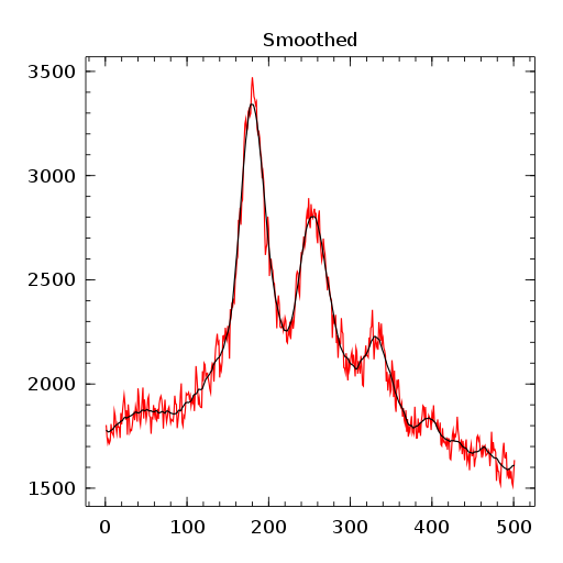
 ")
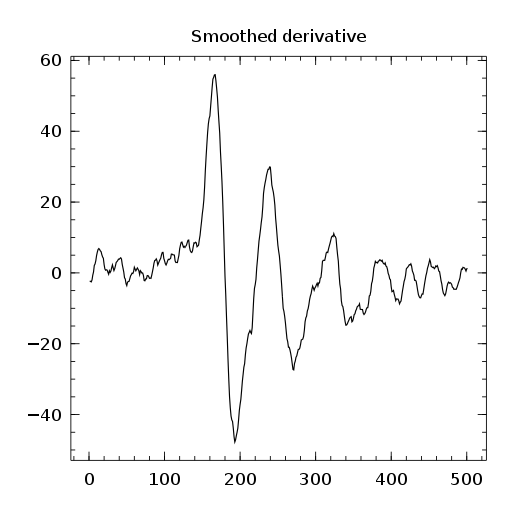
") filter, the second one the smoothed first order derivative
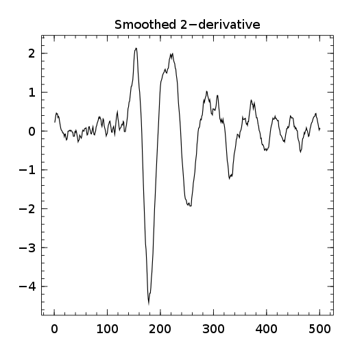
filter, the second one the smoothed first order derivative ") filter and the last one the smoothed second order derivative
filter and the last one the smoothed second order derivative ") filter.
filter. ![\gamma[k]=\sum\limits_i\alpha[i]\beta[k+\lambda i],\ with\ \lambda\in\mathbb{Z}^*](https://s0.wp.com/latex.php?latex=%5Cgamma%5Bk%5D%3D%5Csum%5Climits_i%5Calpha%5Bi%5D%5Cbeta%5Bk%2B%5Clambda+i%5D%2C%5C+with%5C+%5Clambda%5Cin%5Cmathbb%7BZ%7D%5E%2A+&bg=ffffff&%23038;fg=1a1a1a&%23038;s=0 "\gamma[k]=\sum\limits_i\alpha[i]\beta[k+\lambda i],\ with\ \lambda\in\mathbb{Z}^*")
 ,
, 

=1-\frac{\sum\limits_i \min(x_i,y_i)}{\sum\limits_i \max(x_i,y_i)},\ \text{where}\ (x,y)\in\mathbb{R}_+^n\times\mathbb{R}_+^n")
")
![\nabla [(x_1,x_2)\rightarrow max(2.x_1,x_2)]_{x_1=1,x_2=NaN}=(2,0)](https://s0.wp.com/latex.php?latex=%5Cnabla+%5B%28x_1%2Cx_2%29%5Crightarrow+max%282.x_1%2Cx_2%29%5D_%7Bx_1%3D1%2Cx_2%3DNaN%7D%3D%282%2C0%29+&bg=ffffff&%23038;fg=1a1a1a&%23038;s=0 "\nabla [(x_1,x_2)\rightarrow max(2.x_1,x_2)]_{x_1=1,x_2=NaN}=(2,0)")
=\frac{1}{2}(|x+y|-|x-y|)")
=\frac{1}{2}(|x+y|+|x-y|)")
