Re-posted from: https://blog.esciencecenter.nl/10-examples-of-embedding-julia-in-c-c-66282477e62c?source=rss----ab3660314556--julia
A beginner-friendly collection of examples

I have been asked recently about how easy it would be to use Julia from inside C/C++. That was a very interesting question that I was eager to figure out. This question gave me the chance to explore a few toy problems, but I had some issues figuring out the basics. This post aims to help people in a similar situation. I don’t make any benchmarks or claims. Rather, I want to help kickstart future investigations.
The 10 examples in this post are more-or-less ordered by increasing difficulty. I explain some basic bits of Makefile, which can be skipped, if you know what you are doing.
Please notice that this was not done in a production environment, and in no real projects. Furthermore, I use Linux, which is also very specific. I also recommend you to check the code on GitHub, so you see the full result. If possible, leave a star, so I can use it as interest metric.
Target audience
This post should be useful for people evaluating whether using Julia inside C/C++ will be a good idea, or are just very curious about it. I assume some knowledge of Julia and C/C++.
Where is libjulia.so
First, install Julia and remember where you are installing it. I usually use Jill — which is my bash script to install Julia — with the following commands:
In this case, julia will be installed in /opt/julias/julia-x.y.z/ with a link to /usr/local/bin/.
You can try finding out where your Julia is installed using which to find the full path of julia, then listing with -l to check whether that is a link and where it points. For instance,
ls -l $(dirname $(which julia))/julia*
shows all relevant links.
Now, that folder, which I will call JULIA_DIR, should have folders include and lib, and therefore files $JULIA_DIR/include/julia/julia/julia.h and $JULIA_DIR/lib/libjulia.so should exist.
The 10 examples
Now we start with the examples. Since we are using C/C++, I will start from 0, I guess. These examples are some of the files in the GitHub. Look for files sqrtX.cpp, integrationX.cpp, and linear-algebraX.cpp. Notice that there are more files than examples, because some are mostly repetition.
Table of contents
- 0: The basics
- 1: Expanding the basics
- 2: Exceptions
- 3: Including Julia files and callings functions with 4 arguments or more
- 4: C function from Julia from C
- 5: Using a package
- 6: Using the Distributions package
- 7: Creating a class to wrap the Distributions package
- 8: Linear algebra: Arrays, Vectors, and Matrices
- 9: Sparse matrices
0: The basics
Let’s make sure that we can build and run a basic example, taken directly from the official documentation:
I hope the code comments are self-explanatory. To compile this code, let’s prepare a very simple Makefile.
Explaining:
- -fPIC: Position independent code. This is needed because we will work with shared libraries
- -g: Adding debug information because we will probably need it
- JULIA_DIR: It’s out Julia dir!
- -I…: Include path for julia.h
- -L…: Linking path for libjulia.so
- -Wl,…: Linking path for the linker
- -ljulia: libjulia.so
- main.exe: main.cpp: The file main.exe needs the file main.cpp
- On line 7 there must be a TAB, not spaces
- $<: Expands to the left-most requirement (main.cpp)
- $@: Expands to the target (main.exe)
- The Makefile expression as a whole: “To build a main.exe, look for main.cpp and run the command g++ … main.cpp … -o main.exe”
Enter make main.exe in your terminal, and then ./main.exe. Your output should be 1.4142135623730951. I was not expecting this to just work, but it did. I hope you have a similar experience.
1: Expanding the basics
The simplest way to execute anything in Julia is to use jl_eval_string. Variables created using jl_eval_string remain in the Julia interpreter scope, so you can access them:
jl_eval_string("x = sqrt(2.0)");
jl_eval_string("print(x)");
Returned values can be stored as pointers of type jl_value_t. To access their values, use jl_unbox_SOMETYPE. For instance:
jl_value_t *x = jl_eval_string("sqrt(2.0)");
double x_value = jl_unbox_float64(x);
Finally, you can also store pointers to Julia functions using jl_get_function. The returned type is a pointer to a jl_function_t and we can’t just use it as a C++ function. Instead, we will use jl_call1 and jl_box_float64.
jl_function_t *sqrt = jl_get_function(jl_base_module, “sqrt”)
jl_value *x = jl_call1(sqrt, jl_box_float64(2.0));
In the code above we have jl_base_module, which is everything in Base of Julia. The other common module is jl_main_module, which will include whatever we load (using) or create.
The function jl_call1 is used to execute a Julia function with 1 argument. Variants with 0 to 3 arguments also exist, but if you need to call a function with more arguments, you need to use jl_call. We will get to that later.
In the end, we have something like this:
2: Exceptions
Now, try changing the 2.0 in the code above to -1.0. If you call sqrt(-1.0) in Julia you have a DomainError. But if you run the code with the change above, you will have a segmentation fault.
The problem is not in the execution, though, it is in the unboxing below of the now-undefined x. To check for exceptions on the Julia side we can use jl_exception_occurred. It returns the pointer to the error or 0 (NULL), so it can be used in a conditional statement.
To check the contents of jl_exception_occurred, we can use showerror from Julia’s Base.
After calling sqrt of -1.0, add the following:
The first line creates a variable ex and assigns the exception to it. The evaluated expression is the value of ex, which will be either false if there is no exception, or true if something else was returned.
Then, we call showerror from Julia and pass to it Julia’s error stream with jl_strerr_obj(), and the exception. We add some flourish printing before and after the error message.
To call this a few times, we can create a function called handle_julia_exception wrapping it, and move it to auxiliary files (we’ll call them aux.h and aux.cpp). However, since we are printing, we would have to add iostream or stdio to our auxiliary files, and we don’t want that. Instead, what we can do is use jl_printf and jl_stderr_stream to print using only julia.h.
Therefore we can create the following files:
In our main file we can just add #include "aux.h" and call handle_julia_exception() directly. And since we are already here, we can also create a wrapper for jl_eval_string that checks for exceptions as well. Add the following to your auxiliary files:
// To your aux.h
jl_value_t *handle_eval_string(const char* code);
and
// To you aux.cpp
jl_value_t *handle_eval_string(const char* code) {
    jl_value_t *result = jl_eval_string(code);
    handle_julia_exception();
    assert(result && "Missing return value but no exception occurred!");
    return result;
}
And modify your Makefile accordingly:
main.exe: main.cpp aux.o
    g++ $(CARGS) $< $(JLARGS) aux.o -o $@
%.o: %.cpp
    g++ $(CARGS) -c $< $(JLARGS) -o $@
The % in the Makefile acts as a wildcard.
After running the newest version, you should see something like:
Exception:
DomainError with -1.0:
sqrt will only return a complex result if called with a complex argument. Try sqrt(Complex(x)).
I quit!
Other possibilities to handle exceptions and JL_TRY and JL_CATCH but I don’t have an example for it yet.
If you think that example would be useful, leave a comment.
3: Including Julia files and callings functions with 4 arguments or more
Let’s move on to something a little more convoluted, the trapezoid method for computing approximations for integrals.

The idea of the method is to approximate the integral of the function — the blue-shaded region — by a finite amount of trapezoid areas (caveat: the geometric interpretation only applies to positive functions). As the animation suggests, by increasing the number of trapezoids, we tend to get better approximations for the integral.
The neat formula for the approximation is

A basic implementation of the trapezoid method in Julia is as follows:
Don’t worry, we are not allocating when using range, not even when accessing [2:end-1].
Write down this to an aux.jl file and include this file using the code below:
handle_eval_string("include(\"aux.jl\")");
Now we can access trapezoid as any other Julia code, for instance, using jl_eval_string or jl_get_function. It is important to notice that trapezoid is not part of the Base module. Instead, we must use the Main module through jl_main_module.
To test this function, let’s compute the integral of x^2 from 0 to 1. We will use the evaluator to compute x -> x^2, which is the notation for anonymous functions in Julia. The result should be 1/3.
Notice that the function x -> x^2 was created with a handle_eval_string, which calls jl_eval_string. The return value of jl_eval_string is a jl_value_t *, but surprise, a jl_function_t is actually just another name for jl_value_t. The difference is just for readability purposes.
The trapezoid function has 4 arguments, therefore we have to use the general jl_call that we mentioned before. The arguments of jl_call are the function, an array of jl_value_t * arguments, and the number of arguments.
4: C function from Julia from C
How about computing the integral of a C function? We will need to access it through Julia to be able to pass it to a Julia function. First, we must create the function in C. Create a file my_c_func.cpp with the following contents:
It is important that we use extern "C" here, otherwise, C++ will mangle the function name. If you use C instead of C++, then this will not be an issue, but we intend to use C++ down the road. We will compile this code to a shared library, not only a .o object. Therefore, add the following to your Makefile:
lib%.so: %.o
    ld -shared $< -o $@
ld is the linker and -shared is because we want a shared library. Furthermore, you should modify the following:
main.exe: main.cpp aux.o libmy_c_func.so
Now, when you run make main.exe, the libmy_c_func.so library will be compiled.
Finally, to call this function, we use the same string evaluator and Julia’s ccall.
The ccall function has 4+ arguments:
- (:my_c_func, "libmy_c_func.so"): A tuple with the function name and the library;
- Cdouble: Return type;
- (Cdouble,): Tuple with the types of the arguments;
- Then, all the arguments. In this case, only x.
That is it. This change is enough to make the code run. Notice that the function is x^3, so the integral result should be 1 / 4. Those are the only differences in the code.
5: Using a package
Instead of implementing our own integration method, we can use some existing one. One option is QuadGK.jl. To install it, open julia, press ], and enter add QuadGK.
An important note here is that I have not investigated much into maintaining a separate environment for these packages. If you know more about this subject, don’t hesitate to leave a comment.
Here is the code:
handle_eval_string("using QuadGK");
jl_value_t *integrator = handle_eval_string(
    "(f, a, b, n) -> quadgk(f, a, b, maxevals=n)[1]"
);
Just like that we can compute the integral, and compare it with our implementation. Let’s use a harder integral to make things more interesting:

Here is the complete code for this example:
The results you should see are
Integral of 1 / (1 + x^2) is approx: 0.785394
  Error: 4.16667e-06
Integral of 1 / (1 + x^2) is approx: 0.785398
  Error: -1.11022e-16
6: Using the Distributions package
The package Distributions contains various probability-related tools. We are going to use the Normal distributions’ PDF (Probability Density Function) and CDF (Cumulative Density Function) in this example. Don’t worry if you don’t know what these mean, we won’t need to understand the concept, only the formulas.
The Normal distribution with mean Mu (µ) and standard deviation Sigma (σ) has PDF given by

And the CDF of a PDF is

What we will do is use the Distributions package to access the PDF and compute the CDF integral using QuadGK. We will then compare it to the existing CDF function in Distributions.
Once more there is not much secret. You only have to create the Normal structure on the Julia side and use Julia closures to define PDF and CDF jl_function_t with one argument. This is the code:
handle_eval_string("normal = Normal()");
jl_function_t *pdf = handle_eval_string("x -> pdf(normal, x)");
jl_function_t *cdf = handle_eval_string("x -> cdf(normal, x)");
The full code is below
7: Creating a class to wrap the Distributions package
To complicate it a little bit more, let’s create a class wrapping the Distributions package. The basic idea will be a constructor to call Normal , and C++ functions wrapping pdf and cdf. This can be done simply by having a call to handle_eval_string or by creating the function with jl_get_function and calling jl_call_X.
However, to make it more efficient, we want to avoid frequent calls to the functions that deal with strings. One solution is to store the functions returned by jl_get_function and just use them when necessary. To do that, we will use static members in C++.
The two files below show the implementation of our class:
As you can see, we keep a distributions_loaded flag to let the constructor know that the static variables can be used. In the initialization function, we define the necessary functions. The actual implementation of the constructor and the PDF and CDF functions is straightforward.
We can use this new class in our main file easily:
Don’t forget to update your Makefile by replacing aux.o by aux.o Normal.o, i.e., add Normal.o next toaux.o. The result of this execution is
x: -4.00e+00  pdf: +4.97e-08  cdf: +1.12e-08
x: -3.00e+00  pdf: +2.73e-06  cdf: +7.07e-07
x: -2.00e+00  pdf: +8.29e-05  cdf: +2.52e-05
x: -1.00e+00  pdf: +1.39e-03  cdf: +5.11e-04
x: +0.00e+00  pdf: +1.30e-02  cdf: +5.95e-03
x: +1.00e+00  pdf: +6.68e-02  cdf: +4.04e-02
x: +2.00e+00  pdf: +1.90e-01  cdf: +1.64e-01
x: +3.00e+00  pdf: +3.00e-01  cdf: +4.18e-01
x: +4.00e+00  pdf: +2.62e-01  cdf: +7.13e-01
8: Linear algebra: Arrays, Vectors, and Matrices
Let’s start our linear algebra exploration with a matrix-vector multiplication and solving a linear system. We will define the following:

Let’s start with some code:
The first two statements define the vectors and matrices types. Notice that we make explicit that the first has 1 dimension and the second has 2 dimensions.
The next 3 statements allocate the memory for the two vectors x and y, and the matrix A, using the array types we previously defined.
Finally, we have a JL_GC_PUSH3, which informs Julia’s Garbage Collector to not touch this memory. Naturally, we will have to pop these eventually.
Lastly, we declare C arrays pointing to the Julia data. You will notice that AData is a 1-dimensional array because Julia implements dense matrices as a linearized array by columns. That means that the element(i,j) will be at the linearized position i + j * nrows — using 0-based indexing.
To fill the values of the vector x and the matrix A , we can use the code below:
The product of A and x is pretty much the same as any function we had so far.
The noteworthy part of this code is that we have to cast the arrays for jl_value_t * to use them as arguments to jl_call2 , and the output is cast to jl_array_t *. Similarly, we can use jl_array_data(Ax) to access the content of the product.
We can also use mul! to compute the product in place, i.e., without allocating more memory:
Notice that we use jl_main_module because mul! is part of LinearAlgebra .
Finally, we move on to solving the linear system. To do that, let’s use the LU factorization and the ldiv! function. The \ (backslash) operator is usually used here, but we choose ldiv! to solve the linear system in place.
jl_function_t *lu_fact = jl_get_function(jl_main_module, "lu");
jl_value_t *LU = jl_call1(lu_fact, (jl_value_t *) A);
jl_function_t *ldiv = jl_get_function(jl_main_module, "ldiv!");
jl_call3(ldiv, (jl_value_t *) y, LU, (jl_value_t *) Ax);
The last call defines y as the solution of the linear system Ay = (Ax) . Since A is non-singular, we expect y and x to be sufficiently close (numerical errors could appear here). We can verify this using
double *yData = (double *) jl_array_data(y);
double norm2 = 0.0;
for (size_t i = 0; i < n; i++) {
    double dif = yData[i] - xData[i];
    norm2 += dif * dif;
}
cout << "|x - y|² = " << norm2 << endl;
My result was 6.48394e-26 .
To finalize this code, we have to run
JL_GC_POP();
This allows the Julia Garbage Collector to collect the allocated memory. The complete code can be seen below:
9: Sparse matrices
For our next example, we will solve a heat-equation on 1 spatial dimension, using a discretization of time and space called Backward Time Centered Space (BTCS), which is not quick to explain. Check these notes for a thorough explanation.
For our interests, it suffices to say that we will be solving a sparse linear system multiple times, where the matrix is the one below:

We don’t have to store this matrix as a dense matrix (like in the previous example). Instead, we want to store only the relevant elements. To do that, we will create three vectors for the rows and columns indexes, and for the values corresponding to these indexes.
The code is below:
long int rows[3 * n - 2], cols[3 * n - 2];
double vals[3 * n - 2];
for (size_t i = 0; i < n; i++) {
    rows[i] = i + 1;
    cols[i] = i + 1;
    vals[i] = (1 + 2 * kappa);
    if (i < n - 1) {
        rows[n + i] = i + 1;
        cols[n + i] = i + 2;
        vals[n + i] = -kappa;
        rows[2 * n + i - 1] = i + 2;
        cols[2 * n + i - 1] = i + 1;
        vals[2 * n + i - 1] = -kappa;
    }
}
Now, we will create a sparse matrix using the sparse function from the SparseArrays module in Julia. For that, we allocate two array types, one for the integers, and one for the floating point numbers.
On the jl_call3 , we also call jl_ptr_to_array_1d to directly create and return a Julia vector wrapping the data we give it.
The A_sparsematrix is a Julia sparse matrix. Many of the matrix operations that work with dense matrices will work with sparse matrices. To test a different factorization, let’s use the function ldl from the LDLFactorizations package.
Now, we can use ldiv! with ldlObj instead of the LU factorization that we used in the previous example. There is one catch, though. Since we are using the ldlObj “for a while”, we need to prevent the Garbage collector to clean it. But the JL_GC_PUSHX function can only be called once per scope. Therefore, to use it we have to create an internal scope. So something like the following:
The complete code is below:
In the algorithm, we define u as the initial vector, then solve the linear system right u as the right-hand side to obtain unew. Then we assign unew to u and repeat. Each u is an approximation to the solution of the heat equation for a specific moment in time.
You will notice that, in addition to computing the solution, we also plot it using the Plots package. We plot the initial solution at different times. This makes the code much slower, unfortunately. The result can be seen below:

Finalizing and open questions
I hope these 10 examples are helpful to get you started with embedding Julia in C. There are many more things not covered here, in particular things I do not know. Some of them are:
- How to deal with strings?
- How to deal with keyword arguments?
- How to deal with installing packages and environments?
- How to make it faster (e.g., using precompiled images)?
I will be on the lookout for future projects to investigate these. In the meantime, like and follow for more Julia and C/C++ content.
References and extra material
- Embedding Julia in the Julia documentation
- Embedding Julia libraries in C++ by Matthijs Cox
- https://discourse.julialang.org/t/calling-jl-gc-push1-multiple-times/18666
10 examples of embedding Julia in C/C++ was originally published in Netherlands eScience Center on Medium, where people are continuing the conversation by highlighting and responding to this story.
![\gamma[k]=\sum\limits_{i\in\Omega^\alpha}\alpha[i]\beta[k+\lambda i],\text{ with }\lambda\in\mathbb{Z}^*\text{\ \ \ \ \ \ \ \ \ \ \ \ (1)}](https://s0.wp.com/latex.php?latex=%5Cgamma%5Bk%5D%3D%5Csum%5Climits_%7Bi%5Cin%5COmega%5E%5Calpha%7D%5Calpha%5Bi%5D%5Cbeta%5Bk%2B%5Clambda+i%5D%2C%5Ctext%7B+with+%7D%5Clambda%5Cin%5Cmathbb%7BZ%7D%5E%2A%5Ctext%7B%5C+%5C+%5C+%5C+%5C+%5C+%5C+%5C+%5C+%5C+%5C+%5C+%281%29%7D+&bg=ffffff&%23038;fg=1a1a1a&%23038;s=0 "\gamma[k]=\sum\limits_{i\in\Omega^\alpha}\alpha[i]\beta[k+\lambda i],\text{ with }\lambda\in\mathbb{Z}^*\text{\ \ \ \ \ \ \ \ \ \ \ \ (1)}")
 .
.  has been introduced to define:
  convolution
 cross-correlation
 the stationary wavelet transform (the so called
 our vector domain (or support), for instance
![\alpha[i]](https://s0.wp.com/latex.php?latex=%5Calpha%5Bi%5D&bg=ffffff&%23038;fg=1a1a1a&%23038;s=0 "\alpha[i]") is defined for
is defined for
\text{ and }i_{\max}=u(\Omega^\alpha)")
 the scaled domain
}") and
and }")
 the relative complement of
  with respect to the set
  defined by
 \wedge (i\notin B) \}")
 , it is sufficient to introduce the left and right parts (that can be empty)
 _{\text{Left}}=\llbracket l(A), \min{(u(A),l(B)-1)} \rrbracket")
_{\text{Right}}=\llbracket \max{(l(A),u(B)+1)}, u(A) \rrbracket")
 ,
,  defined on
  ,
,  we want to define and implement an algorithm that computes
 ![\gamma[k]](https://s0.wp.com/latex.php?latex=%5Cgamma%5Bk%5D&bg=ffffff&%23038;fg=1a1a1a&%23038;s=0 "\gamma[k]") for
for  .
.  the domain that does not violate
\Leftrightarrow (\forall i \in \Omega^\alpha \Rightarrow l(\Omega^\beta)-\lambda i \le k \le u(\Omega^\beta)-\lambda i)")
-\lambda i \le k \le \min\limits_{i\in \Omega^\alpha} u(\Omega^\beta)-\lambda i")
-l(\lambda \Omega^\alpha) \le k \le u(\Omega^\beta)-u(\lambda \Omega^\alpha)")
-l(\lambda \Omega^\alpha) , u(\Omega^\beta)-u(\lambda \Omega^\alpha) \rrbracket }")
![\gamma[k],\ k\in\Omega^\gamma](https://s0.wp.com/latex.php?latex=%5Cgamma%5Bk%5D%2C%5C+k%5Cin%5COmega%5E%5Cgamma&bg=ffffff&%23038;fg=1a1a1a&%23038;s=0 "\gamma[k],\ k\in\Omega^\gamma") (Eq. 1) is splitted into two parts:
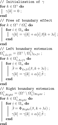
(Eq. 1) is splitted into two parts:  free of boundary effect,
 that requires boundary extension
 ")
![\beta[.]](https://s0.wp.com/latex.php?latex=%5Cbeta%5B.%5D&bg=ffffff&%23038;fg=1a1a1a&%23038;s=0 "\beta[.]") and are sometimes entailed by a validity condition. For a better clarity I give explicit lower/upper bounds:
and are sometimes entailed by a validity condition. For a better clarity I give explicit lower/upper bounds: 
")
")
![\tilde{\beta}_j = \beta[2\,j_{min}-j]](https://s0.wp.com/latex.php?latex=%5Ctilde%7B%5Cbeta%7D_j++%3D+%5Cbeta%5B2%5C%2Cj_%7Bmin%7D-j%5D&bg=ffffff&%23038;fg=1a1a1a&%23038;s=0 "\tilde{\beta}_j = \beta[2\,j_{min}-j]")

![\tilde{\beta}_j = \beta[j_{max}-j_{min}+j+1]](https://s0.wp.com/latex.php?latex=%5Ctilde%7B%5Cbeta%7D_j+%3D++%5Cbeta%5Bj_%7Bmax%7D-j_%7Bmin%7D%2Bj%2B1%5D&bg=ffffff&%23038;fg=1a1a1a&%23038;s=0 "\tilde{\beta}_j = \beta[j_{max}-j_{min}+j+1]")

![\tilde{\beta}_j = \beta[j_{min}]](https://s0.wp.com/latex.php?latex=%5Ctilde%7B%5Cbeta%7D_j+%3D+%5Cbeta%5Bj_%7Bmin%7D%5D&bg=ffffff&%23038;fg=1a1a1a&%23038;s=0 "\tilde{\beta}_j = \beta[j_{min}]")

")
")
![\tilde{\beta}_j = \beta[2\,j_{max}-j]](https://s0.wp.com/latex.php?latex=%5Ctilde%7B%5Cbeta%7D_j++%3D+%5Cbeta%5B2%5C%2Cj_%7Bmax%7D-j%5D&bg=ffffff&%23038;fg=1a1a1a&%23038;s=0 "\tilde{\beta}_j = \beta[2\,j_{max}-j]")

![\tilde{\beta}_j = \beta[-j_{max}+j_{min}+j-1]](https://s0.wp.com/latex.php?latex=%5Ctilde%7B%5Cbeta%7D_j+%3D+%5Cbeta%5B-j_%7Bmax%7D%2Bj_%7Bmin%7D%2Bj-1%5D&bg=ffffff&%23038;fg=1a1a1a&%23038;s=0 "\tilde{\beta}_j = \beta[-j_{max}+j_{min}+j-1]")

![\tilde{\beta}_j = \beta[j_{max}]](https://s0.wp.com/latex.php?latex=%5Ctilde%7B%5Cbeta%7D_j+%3D+%5Cbeta%5Bj_%7Bmax%7D%5D&bg=ffffff&%23038;fg=1a1a1a&%23038;s=0 "\tilde{\beta}_j = \beta[j_{max}]")
 we want to define a periodic function
  of period
  . This function must fulfills the
 ![\tilde{\beta}[j+T]=\tilde{\beta}[j]](https://s0.wp.com/latex.php?latex=%5Ctilde%7B%5Cbeta%7D%5Bj%2BT%5D%3D%5Ctilde%7B%5Cbeta%7D%5Bj%5D&bg=ffffff&%23038;fg=1a1a1a&%23038;s=0 "\tilde{\beta}[j+T]=\tilde{\beta}[j]") relation.
relation. ") where
where=\bmod_F(j,U+1)")
 is the modulus function associated to a
  , we first translate the indices
=j-j_{\min}")
}_{j_{\min}}=\tau_{-j_{\min}}")

}_{j_{\min}} \circ \phi^P_{j_{\max}- j_{\min}} \circ \tau_{j_{\min}}")
}")
 using
using  with
with=U-|U-j|")
![\tilde{\beta}[U-j]=\tilde{\beta}[U+j]](https://s0.wp.com/latex.php?latex=%5Ctilde%7B%5Cbeta%7D%5BU-j%5D%3D%5Ctilde%7B%5Cbeta%7D%5BU%2Bj%5D&bg=ffffff&%23038;fg=1a1a1a&%23038;s=0 "\tilde{\beta}[U-j]=\tilde{\beta}[U+j]") relation for
relation for  .
.  using
using  (attention
  and not
  , otherwise the component
  is duplicated!).
}_{j_{\min}} \circ \phi^M_{j_{\max}- j_{\min}} \circ \phi^P_{2(j_{\max}- j_{\min})-1} \circ \tau_{j_{\min}}")
)| }")
![\tilde{\beta}=\Phi(\beta,k+\lambda i)=\beta[\phi^X[k+\lambda i]]](https://s0.wp.com/latex.php?latex=%5Ctilde%7B%5Cbeta%7D%3D%5CPhi%28%5Cbeta%2Ck%2B%5Clambda+i%29%3D%5Cbeta%5B%5Cphi%5EX%5Bk%2B%5Clambda+i%5D%5D+&bg=ffffff&%23038;fg=1a1a1a&%23038;s=0 "\tilde{\beta}=\Phi(\beta,k+\lambda i)=\beta[\phi^X[k+\lambda i]]")
 is the boundary extension you have chosen (periodic, constant
 ). You do not have to take care of any validity condition, these formula are general.
  (access memory in the right order), use simd, or C++ meta-programming with loop unrolling for fixed
 in Julia, Fortran
 defined on
  (Julia) or
  (C++).
  .
. ![\alpha[i] = \tilde{\alpha}[\tilde{i}] = \tilde{\alpha}[i-l(\Omega^\alpha)+\tilde{i}_0]](https://s0.wp.com/latex.php?latex=%5Calpha%5Bi%5D+%3D++%5Ctilde%7B%5Calpha%7D%5B%5Ctilde%7Bi%7D%5D+%3D+%5Ctilde%7B%5Calpha%7D%5Bi-l%28%5COmega%5E%5Calpha%29%2B%5Ctilde%7Bi%7D_0%5D+&bg=ffffff&%23038;fg=1a1a1a&%23038;s=0 "\alpha[i] = \tilde{\alpha}[\tilde{i}] = \tilde{\alpha}[i-l(\Omega^\alpha)+\tilde{i}_0]")
![\gamma[k]=\sum\limits_{i\in\Omega^\alpha}\alpha[i]\beta[k+\lambda i] = \sum\limits_{i\in\Omega^\alpha}\tilde{\alpha}[i-l(\Omega^\alpha)+\tilde{i}_0]\beta[k+\lambda i]](https://s0.wp.com/latex.php?latex=%5Cgamma%5Bk%5D%3D%5Csum%5Climits_%7Bi%5Cin%5COmega%5E%5Calpha%7D%5Calpha%5Bi%5D%5Cbeta%5Bk%2B%5Clambda+i%5D+%3D+%5Csum%5Climits_%7Bi%5Cin%5COmega%5E%5Calpha%7D%5Ctilde%7B%5Calpha%7D%5Bi-l%28%5COmega%5E%5Calpha%29%2B%5Ctilde%7Bi%7D_0%5D%5Cbeta%5Bk%2B%5Clambda+i%5D+&bg=ffffff&%23038;fg=1a1a1a&%23038;s=0 "\gamma[k]=\sum\limits_{i\in\Omega^\alpha}\alpha[i]\beta[k+\lambda i] = \sum\limits_{i\in\Omega^\alpha}\tilde{\alpha}[i-l(\Omega^\alpha)+\tilde{i}_0]\beta[k+\lambda i]")
+\tilde{i}_0") we have
we have-l(\Omega^\alpha)+\tilde{i}_0 \rrbracket")
 - \tilde{i}_0)}_{\beta\_\text{offset}}")
![\boxed{ \gamma[k]=\sum\limits_{\tilde{i}=\tilde{i}_0}^{u(\Omega^\alpha)-l(\Omega^\alpha)+\tilde{i}_0}\tilde{\alpha}[\tilde{i}]\beta[k+ \lambda \tilde{i} + \lambda (l(\Omega^\alpha) - \tilde{i}_0)]}](https://s0.wp.com/latex.php?latex=%5Cboxed%7B+%5Cgamma%5Bk%5D%3D%5Csum%5Climits_%7B%5Ctilde%7Bi%7D%3D%5Ctilde%7Bi%7D_0%7D%5E%7Bu%28%5COmega%5E%5Calpha%29-l%28%5COmega%5E%5Calpha%29%2B%5Ctilde%7Bi%7D_0%7D%5Ctilde%7B%5Calpha%7D%5B%5Ctilde%7Bi%7D%5D%5Cbeta%5Bk%2B+%5Clambda+%5Ctilde%7Bi%7D+%2B+%5Clambda+%28l%28%5COmega%5E%5Calpha%29+-+%5Ctilde%7Bi%7D_0%29%5D%7D+&bg=ffffff&%23038;fg=1a1a1a&%23038;s=0 "\boxed{ \gamma[k]=\sum\limits_{\tilde{i}=\tilde{i}_0}^{u(\Omega^\alpha)-l(\Omega^\alpha)+\tilde{i}_0}\tilde{\alpha}[\tilde{i}]\beta[k+ \lambda \tilde{i} + \lambda (l(\Omega^\alpha) - \tilde{i}_0)]}")
 other arrays are less problematic:
  - 1 \rrbracket") . This does not reduce the generality of the subroutine.
. This does not reduce the generality of the subroutine. which is the output array, as for
  - 1 \rrbracket") , but we provide
, but we provide  - 1 \rrbracket") to define the components we want to compute. The other components,
to define the components we want to compute. The other components,  - 1 \rrbracket \setminus \Omega^\gamma") , will remain unmodified by the subroutine.
, will remain unmodified by the subroutine.
 -1 \rrbracket")
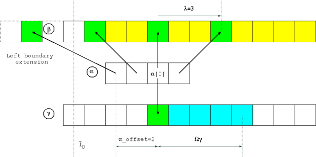
 you are in the “usual situation”. If you have a window size of
  , taking
  returns the middle of the window. Here, in the Fig. below, the graphical representation of an arbitrary case: a filter if size
  , with
  and
and  .
. 
 operator.

 arrays (not
  ones): some conjugation are missing
 domain
\in \Omega^\alpha \times \Omega^\beta") .
. 
-u(\lambda \Omega^\alpha) , u(\Omega^\beta)-l(\lambda \Omega^\alpha) \rrbracket }")
 domain
 what is the domain of
 =\Omega^\gamma")
-u(\lambda \Omega^\alpha) , u(\Omega^\beta_{2'})-l(\lambda \Omega^\alpha) \rrbracket = \llbracket l(\Omega^\gamma),u(\Omega^\gamma) \rrbracket")
+u(\lambda \Omega^\alpha),u(\Omega^\gamma)+l(\lambda \Omega^\alpha) \rrbracket }")

=1-\frac{\sum\limits_i \min(x_i,y_i)}{\sum\limits_i \max(x_i,y_i)},\ \text{where}\ (x,y)\in\mathbb{R}_+^n\times\mathbb{R}_+^n")
")
![\nabla [(x_1,x_2)\rightarrow max(2.x_1,x_2)]_{x_1=1,x_2=NaN}=(2,0)](https://s0.wp.com/latex.php?latex=%5Cnabla+%5B%28x_1%2Cx_2%29%5Crightarrow+max%282.x_1%2Cx_2%29%5D_%7Bx_1%3D1%2Cx_2%3DNaN%7D%3D%282%2C0%29+&bg=ffffff&%23038;fg=1a1a1a&%23038;s=0 "\nabla [(x_1,x_2)\rightarrow max(2.x_1,x_2)]_{x_1=1,x_2=NaN}=(2,0)")
=\frac{1}{2}(|x+y|-|x-y|)")
=\frac{1}{2}(|x+y|+|x-y|)")
