By: Jacob Quinn
Re-posted from: https://quinnj.home.blog/2019/07/21/a-tour-of-the-data-ecosystem-in-julia/
Julia 1.0 was released at JuliaCon 2018 and it’s been a quick year for the package ecosystem to build upon the first long-term stable release. In a lot of ways, pre-1.0 for packages involved a lot of experimentation; a lot of trying out various ideas, shotgun-style and seeing what sticks, in addition to trying to keep up with the evolving core language. One of my favorite things about Julia is the great efforts that have been made to collaborate, coordinate, and modularize not just the base language and standard libraries, but the entire package ecosystem. Julia was born in the age of GitHub, Discourse, and Slack, which has led to an exceptional amount of public communication from and with core developers, targeted efforts to automatically update package code and test the impact of core changes to the ecosystem, and a proliferation of user-group meetups and domain-specific GitHub organizations. I don’t feel dishonest in saying I think Julia is the most collaborative programming language that exists today.
With all this context, one might be wondering: so what is the current status of working with data in Julia? How do various packages like CSV.jl, DataFrames.jl, JuliaDB.jl, and Query.jl play together. And so I present, “A Tour of the Data Ecosystem in Julia”. Let’s begin…
Data I/O: How do I get data in and out of Julia?
Text Files
I once heard Jeff Bezanson say tongue-in-cheek, “It doesn’t really matter what fancy features you put in a programming language, all people really want to do is read csv files. That’s it, just csv file reading.” Julia has grown a lot since the earliest days of dlmread, with several excellent packages for reading csv and other delimited files, each growing out of a unique idea for approaching this old problem or addressing a specific integration need.
CSV.jl
As blog author, you’ll have to forgive the shameless plug for my own packages: I started CSV.jl in 2015 to try and make a strong effort to match csv parsing functionality provided by other popular languages (in particular, Pandas and fread in R). Since then, it’s accumulated some ~400 commits from over 25 collaborators, and recently hit issue #464. It also released a significant upgrade with the recent 0.5 release, bringing performance inline with the fastest parsers in other languages, while providing some powerful and unique features not available elsewhere, including: “perfect” column typing without needing to restart parsing at all, auto delimiter detection, automatic handling of invalid rows, and several options/layers for lazily parsing files, all with unparalleled performance (a full feature comparison with pandas and R can be found in the latest discourse announcement post). Part of CSV.jl’s speed comes from the hand-tuned type parsers made available in the Parsers.jl package, which includes extremely performant parsing for ints, floats, bools, and dates/datetimes, all in pure Julia.
Tables.jl
We’re going to take a quick detour from I/O packages here to mention a key building block in the I/O story. The Tables.jl package was born during the 2018 JuliaCon hack-a-thon. It was a collaboration between several data-related package authors to come up with essentially two access patterns for “table” like data: “rows” and “columns”. The core idea is simple, yet powerful: any table-like data format that can implement one of the access patterns (via row iteration, or column access), can “automatically” integrate with any downstream package that then uses one of the access patterns, all without needing to take bi-directional dependencies. Even being a relatively new package, the power of this interface can be seen already in the integrations already available:
- In-memory datastructures
- DataFrames.jl
- TypedTables.jl
- IndexedTables.jl/JuliaDB.jl
- FunctionalTables.jl
- Data Formating/Processing Packages
- DataKnots.jl
- FreqTables.jl
- Mustache.jl
- FormattedTables.jl
- PrettyTables.jl
- TableView.jl
- BrowseTables.jl
- Data File Format Packages
- CSV.jl
- Feather.jl
- StataDTAFiles.jl
- Taro.jl
- XLSX.jl
- Database Packages
- ODBC.jl
- SQLite.jl
- MySQL.jl
- LibPQ.jl
- JDBC.jl
- Statistics Packages
- StatsModels.jl
- MLJ.jl
- GLM.jl
- Plotting Packages
- StatsMakie.jl
- StatsPlots.jl
- TableWidgets.jl
Ok, back to data I/O. We also have the wonderful TextParse.jl, which started as the data ingestion engine for JuliaDB.jl. While blazing fast, it doesn’t have quite the maturity or breadth of functionality compared to CSV.jl, like this long-standing issue of incorrect float parsing. The CSVFiles.jl package also exists to provide FileIO.jl integration, meaning you can just do load("data.csv") and FileIO.jl automatically recognizes the .csv extension and knows how to load the data. (A full feature comparison between CSV.jl and CSVFiles.jl can be found here). Another interesting approach to csv reading popped up recently in the form of TableReader.jl from the ever-talented Kenta Sato, using finite state machines. A pretty decent collection of benchmarks can be found here.
In addition to the excellent packages for handling text-based, delimited files, there are also some great files for managing/handling data formats in general.
- RData.jl: for reading
.rdafiles from R into Julia - DBFTables.jl: for reading
.dbffiles into Julia - StatFiles.jl: for reading SAS, SPSS, and Stata files into Julia
- StataDTAFiles.jl: for reading and writing Stata files
- DataDeps.jl: for declaring data dependencies and managing reproducible setups for with data in Julia
- ExcelFiles.jl: for reading excel files into Julia and integration with FileIO.jl
Another popular option for data storage is binary-based formats, including feather, apache arrow, parquet, orc, avro, and BSON. Julia has pretty good coverage of these formats, including native Julia implementations in Feather.jl (and FileIO.jl integration in FeatherFiles.jl), Arrow.jl, and Parquet.jl (again, with FileIO.jl integration with ParquetFiles.jl). There’s also the BSON.jl package for binary JSON support. Beginning support for avro has been started in Avro.jl, and I’m personally interested in diving into the ORC format.
Database Support
As mentioned above in Tables.jl integrations, there are also great packages in place to support extracting data from databases, including:
- ODBC.jl: provides generic support for any database that provides a compatible ODBC driver. Supports parameterized queries for inserting data, as well as extracting data from a query, and with Tables.jl support, “exporting” the results to any Tables.jl-compatible sink. It does require setting up an ODBC administrator tool on OSX and linux (windows has builtin support), and then proper setup/installation of the specific database’s ODBC driver, but once setup, things generally work pretty seamlessly.
- JDBC.jl: the JDBC.jl package also provides access for databases that support JDBC access. It does so via JavaCall.jl, which does require an active JDK to work, which can also be tricky to setup, but database vendors tend to have pretty good support for a JDBC driver
- MySQL.jl/LibPQ.jl: specific packages for mysql/postgres databases, respectively. Both provide integration with Tables.jl and aim to provide support for database-specific types and functionality (beyond the more generic interfaces of ODBC/JDBC). They can be easier to setup since there’s no “middle man” interface library and you just need to interact with the database libraries directly.
- SQLite.jl: a library providing integration with the excellent sqlite database; supports in-memory databases as well as file-based. Supports parameterized queries and Tables.jl integration for loading data and extracting query results.
Data Processing: what can I do with my data once it’s in Julia?
Once you identify the right I/O package for reading your data, you then have a choice to make with regards to what you need/want to do with it. Clean it? Reshape it? Filter/calculate/group/sort it? Just browse around for a little while? Do advanced statistics, model training, or other machine learning techniques? Here we take a tour of the current landscape of packages that provide various types of functionality with regards to data processing, including table-like structures, query functionality, and statistics/machine learning.
Table Structures
Yes, in Julia we can have an entire section where we talk about table structures, plural. Sometimes when I mention to people that there are several dataframe-like packages in Julia, they are initially confused: why does Julia need more than one table package? Why doesn’t everyone just work on a single package to focus on quality over quantity? My most common response goes something like this: for a project like Pandas, or data.table, or data.frame, most of the actual code is written in what language? Python? Or R? It’s actually C/C++. The common belief is that because R/Python are dynamic, “high-level” languages, they can’t be fast, but that’s no worry, you just write the parts that need to be fast in C. But therein lies a core issue: for languages like Python and R, where the user-to-developer ratio is so high, having core pieces of functionality written in a lower-level language like C makes the code much less accessible to someone who wants to contribute, let alone just take a peek under the hood to see how things work. It automatically splits the code into a lower-level “black box” component, and a higher-level “wrapper” component. I believe it stunts innovation due to such a high “barrier to entry” to take a new approach to a table structure. I might be a budding R or Python user, getting into developing things, but shoot, if I want to make a meaningful contribution to Pandas or data.table, all the sudden I’m wading into deep make/cmake/build issues, compiler versions, and manual memory management that I’ve never dealt with before. The other alternative is I write something in pure R/Python which will just surely be doomed to performance issues, regardless of how novel my interfaces or APIs might be.
Julia, however, is a famously declared solution to this “two-language problem”. No longer do budding developers need to fear plain for-loops, or vectorize every operation, or rely on C/C++ for the “core stuff”. You can just write plain Julia, down in the trenches, and up at the highest-level user APIs. Julia, all the way down.
I firmly believe this has led to greater innovation in Julia for experimenting with unique table structures, as well as making packages more accessible to those hoping to contribute.
Ok, enough soap-boxing, let’s talk packages.
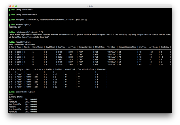
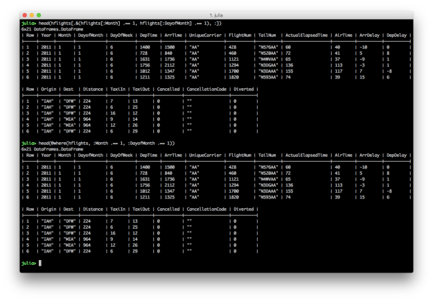
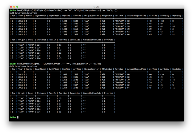
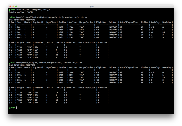
DataFrames.jl
The DataFrames.jl package is one of the very oldest packages in the Julia ecosystem. This tenure and naming proximity with its cousins in Pandas and R have also made it one of the most popular packages for those hoping to give Julia a try. The package has evolved quite a bit since its early days, and is rapidly approaching its own 1.0 release (expected around JuliaCon 2019). Development over the last year or two has focused on core performance, safety of APIs, and overall consistency with Base APIs. The amount of thought, effort, discussion, and documentation by numerous collaborators makes it the most mature “table” package in my opinion. So what’s unique about DataFrames? I’ll try to give what I deem to be notable highlights of how DataFrames.jl approaches representing tabular data:
- A
DataFramestores columns internally as aVector{AbstractVector}; but wait, you might ask, isn’t that type unstable (since we’re essentially lumping all columns, regardless of individual column type, asAbstractVector)? Yes! And on purpose! Experienced Julia developers are quick to point out that sometimes code can get “overly typed”, leading to “compilation overdrive”, where the compiler is having to generate very specialized code for every operation, with compiled code reuse rare. ADataFramecan represent any number of columns, with any combination of column types, so it’s a natural scenario where you may want to “hide” too much type information from the compiler by slapping the lowest common denominator abstract type as the type label (AbstractVectorin this case). This design decision has certainly been extensively discussed, but remains as-is, if not as a more compiler-friendly option than other “strongly typed table” types. - DataFrames.jl includes specialized subtypes for representing
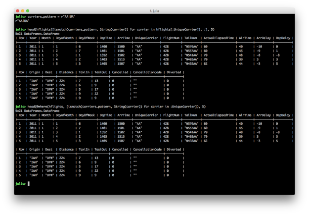
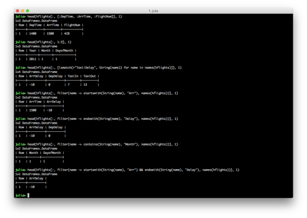
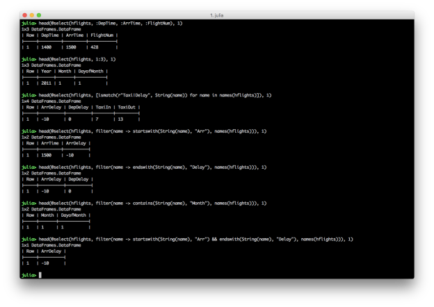
SubDataFrames andGroupedDataFrames, as opposed to returning fullDataFrames; these “lazy” structures are mostly used in intermediate operations and is a useful way to avoid too much unnecessary data copying/movement - Core manipulation operations included in the package itself include grouping, joining, and indexing; in particular, supporting column indexing via regex matches, functional selecting,
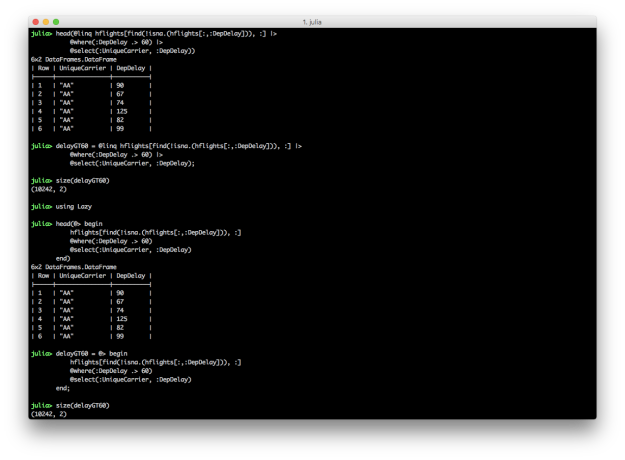
Notindexing (inverted indices), and flexible interfaces similar toBase.Arrays in terms of filtering/selecting specific indices for rows or columns. - A lot of work in recent years has also been to simplify and move code out of the DataFrames.jl package, to focus on the core types, functionality, and reduce the dependency burden, being a common dependency for packages around the ecosystem; this has included notably the creation of the DataFramesMeta.jl package to support other common query/filter/manipulation operations
- DataFrames.jl supports the Tables.jl interface, which means any I/O package also supporting it can automatically convert it’s table format into an in-memory DataFrame, and convert back to the format for output
IndexedTables.jl / JuliaDB.jl
JuliaDB.jl splashed onto the Julia scene in early 2017, touting a new approach to query/table operations that utilized type stability and Julia’s built in parallelism to provide “out of core” functionality like a database. JuliaDB.jl’s core table type actually lives in the IndexedTables.jl package, which in turn uses the clever StructArrays.jl package to turn NamedTuple rows into an efficient struct-of-arrays structure more suitable for columnar analytics. JuliaDB.jl itself then, with the use of Dagger.jl, adds the “parallel” layer on top of IndexedTables.jl. The benefits of “type stability” come from a table being essentially encoded as Table{Col1T, Col2T, Col3T, ...}, where the full type of each column is encoded in the top-level table type. This allows operations like selecting columns, filtering, and aggregating to be extremely efficient due to the compiler knowing the exact types it’s dealing with (as opposed to having to do “runtime” checks like in the DataFrames.jl case). Now, as discussed in the DataFrames.jl section, this doesn’t come without a cost; indeed, there’s a long-standing issue for dealing with the compilation cost for tables with a large number of columns. But, in the case of a manageable number of columns, and with the ability to scale tables up beyond a single machine’s memory limits is powerful functionality. JuliaDB.jl is also sponsored by JuliaComputing, which gives it a nice stamp of support and stability. While it may lack some of the maturity of DataFrames.jl long-discussed APIs, I’m excited by the unique, “Julian” approach JuliaDB.jl provides in the big data analytics space. Go check out the docs here and give it a spin. An additional package providing experimental manipulation functions for JuliaDB is JuliaDBMeta.jl, which mostly mirrors the before-mentioned DataFramesMeta.jl, but for JuliaDB tables.
TypedTables.jl
The TypedTables.jl package is one that started out in “experimentation” mode for a while until recently being declared “ready” by its primary author, the venerable Andy Ferris. Andy has long been known in the Julia community for his eye for API consistency and being able to strike that elusive balance between theoretical ideals and practical use. In TypedTables.jl, the “fully type stable” approach is taken, similar to IndexedTables.jl/JuliaDB.jl, with a Table being defined literally as <: AbstractVector{T} where {T <: NamedTuple}, that is, a collection of “rows” or NamedTuples. While TypedTables.jl includes two @Select and @Compute macros for simple manipulations, some of the more interesting promise comes from the TypedTables.jl “supporting cast” packages:
- AcceleratedArrays.jl: a tidy package to turn any array into an “indexed” array (in the database sense), to provide optimized “search” functions:
findall,findfirst,filter,unique,group,join, etc. AnAcceleratedArraycan thus be used in a TypedTable to provide powerful indexing behavior for an entire table (though note that it works on anyAbstractArray, which means these indexed columns could even be used in a DataFrame). - SplitApplyCombine.jl: this package provides a powerful set of functions to perform common split, apply, and combine operations on generic collections like
mapmany,group,product,groupreduce, andinnerjoin. The aim is to provide the basic building blocks of relational algebra functions that work on any kind of collection, obviously including a TypedTable as a specialized type of AbstractVector of NamedTuples.
CSV.File
One more honorable mention for table structures (and another shameless plug) actually comes from the CSV.jl package. While CSV.read materializes a file as a DataFrame, a CSV.File, which supports all the same keyword arguments as CSV.read, can be used to transfer data to any other Tables.jl sink, or used itself as a table directly. It supports getproperty for column view access and iterates a CSV.Row type (which acts like a NamedTuple). I think as packages continue to evolve, we’ll see more and more cases of customized structures like this, which allow for certain efficiencies or specialized views into raw data formats, and with sufficiently general interfaces like Tables.jl and SplitApplyCombine.jl, users won’t need to worry as much about conforming to a single table structure for everything, but can focus on understanding more generic interfaces, and using data structures optimized for specific use-cases, data formats, and workflows.
Query.jl
Another package (set of packages really) that must be discussed in the Julia data ecosystem is Query.jl. Pioneered by David Anthoff, Query.jl provides a LINQ implementation for Julia. Query.jl and its sister package QueryOperators.jl provide a custom “query dsl” by a set of macros that allow convenient “query context” syntax for common manipulation tasks: selection and projection, filtering, grouping, and joining. These “query verbs” also are able to operate on any iterator, in true LINQ fashion, which makes the processing functions extremely versatile. While currently Query.jl/QueryOperators.jl hold the sole implementations of the query verbs, the grander scheme of having a custom dsl is the ability to represent entire queries in an AST (abstract syntax tree), which could then allow custom implementations that “execute” a structured query. This is most immediately useful when one considers being able to use a single “query dsl” to operate on both DataFrames and database tables, having a query translated into a vendor-specific SQL syntax. While not currently fully fleshed out, the ambitious undertaking is exciting to track.
DataValues.jl
One note for users on the use of Query.jl is the current reliance on the DataValues.jl package to represent missing data. What that means is that query functions in Query.jl/QueryOperators.jl aren’t integrated with the Base-builtin representation of missing, but rely on the DataValues.jl package, which defines a DataValue{T} wrapper type that also holds whether a value is missing or not (along with what “type” of missing value it is). While the history of missing data in Julia is long and storied, Andy Ferris wisely noted that no missing value representation is perfect. missing was included in Base largely due to the ease of working with a single sentinel value, and compiler support for code generation involving Union{T, Missing}. Inherent in the use of Union{T, Missing}, however, is a current compiler complexity involving inference of Union values that are stored in a parametric struct field. This affects the @map macro in Query.jl with NamedTuple inputs to NamedTuple outputs, hence, Query.jl relies on the use of DataValue{T} to more conveniently pass type information through projections. There are also active efforts explore ways the core language can avoid the need for an explicit wrapper type while still propagating the type information soundly through projections.
Additional Data Efforts
Other efforts integrating with the data ecosystem include (but are certainly not limited to):
- StatsModels.jl: for specifying (in familiar “formula” notation), fitting and evaluating statistical models; can operate on any Tables.jl-compatible
- GLM.jl for working specifically with generalized linear models
- LightQuery.jl: another budding approach to type-stable querying capabilities
- Flux.jl for an extremely extensible approach to machine learning modelling, GPU integration, and pure Julia, all the way down
- Distributions.jl: for sampling, moments, and density/mass functions for a wide variety of distributions
- StatsMakie.jl for GPU-enabled statistical plotting goodness
- MLJ.jl: another new holistic approach to representing a variety of machine learning models sponsored by the Alan Turing Institute
- ScikitLearn.jl for Julia access to the scikit-learn APIs for machine learning, including pure Julia implementations and integration with python models via PyCall.jl
- OnlineStats.jl: a mature, fully featured statistical package for “online” statistical algorithms, including well-documented source code for published algorithms
- TextAnalysis.jl: providing algorithms, statistical support, and feature engineering for text analysis
- Dagger.jl: a dask-like Julia framework for distributed, parallel computation graphs
- MultivariateStats.jl: stats, but for multiple variables!
- RCall.jl: package that allows integrating with the R statistical language; transfer objects between languages, call R functions/libraries, etc.
- StatsPlots.jl: another strong statistical plotting package
Future of Data in Julia
So now JuliaCon 2019 is upon us and we have to wonder: what’s next for working with data in Julia? As I’ve tried to illustrate in this long showcase of Julia packages, the data ecosystem has come along way since the official 1.0 release of the language itself. Support for the most common data formats is about as mature as any other language, but there’s always room to improve. The in-memory processing is an exciting space to watch in Julia due to the number of approaches being fleshed out, with varying degrees of maturity. DataFrames.jl is solid and should be a main utility knife for any Julia programmer, but one of the wonders of Julia, as mentioned above, is the ease of developing high-level, performant solutions in the language itself, so it’s exciting to see alternative approaches that can offer trade-offs or additional features that may enable better workflows depending on the environment. But given all that, here’s a shortlist of things swimming in my head around the future of the data ecosystem in Julia:
- Ensure the performance and usability of
Union{T, Missing}to represent missing data in Julia; currently, 95% of uses and workflows work amazingly well, but we always want to track down corner cases and do everything we can to improve the compiler, core language, or APIs to improve - Data format support: the job is never done here, but on my mind are an officially blessed (and integrated) implementation of apache arrow, write support for Parquet.jl, and a Julia package for supporting the ORC data format
- Working towards a common API package/definitions for common table processing tasks; while exploratory efforts are always encouraged, it could be immensely convenient to users of various table types if there were a common set of operations that “just worked”. While Query.jl currently provides the best solution for this, it has other integration issues in the ecosystem; so working to resolve those or define a new common “table operations” type package
- Relatedly, defining a full “structured query graph” model could be one way to provide a lower-level shared representation of querying tasks. This could catalyze “frontend” efforts (custom DSLs like Query.jl’s, or new dplyr-like verbs, or even a plain SQL parsing package) to “lower” to this common representation, while allowing similar types of backend innovation in *how* these structured query graphs are executed (with parallel support, out-of-core, etc.). I’ve recently been studying an old effort to do something like this for inspiration
For those who made it this far, kudos! As always, follow and ping me on twitter to chat data in Julia. And if you’ll be at JuliaCon 2019 in Baltimore, hit me up in the official Julia slack to meet up and chat.