By: Clinton Brownley
Re-posted from: https://cbrownley.wordpress.com/2017/11/29/data-wrangling-in-julia-based-on-dplyr-flights-tutorials/
A couple of my favorite tutorials for wrangling data in R with dplyr are Hadley Wickham’s dplyr package vignette and Kevin Markham’s dplyr tutorial. I enjoy the tutorials because they concisely illustrate how to use a small set of verb-based functions to carry out common data wrangling tasks.
I tend to use Python to wrangle data, but I’m exploring the Julia programming language so I thought creating a similar dplyr-based tutorial in Julia would be a fun way to examine Julia’s capabilities and syntax. Julia has several packages that make it easier to deal with tabular data, including DataFrames and DataFramesMeta.
The DataFrames package provides functions for reading and writing, split-apply-combining, reshaping, joining, sorting, querying, and grouping tabular data. The DataFramesMeta package provides a set of macros that are similar to dplyr’s verb-based functions in that they offer a more convenient, readable syntax for munging data and chaining together multiple operations.
Data
For this tutorial, let’s following along with Kevin’s tutorial and use the hflights dataset. You can obtain the dataset from R with the following commands or simply download it here: hflights.csv
install.packages("hflights")

library(hflights)

write.csv(hflights, "hflights.csv")
Load packages and example dataset
To begin, let’s start the Julia REPL, load the DataFrames and DataFramesMeta packages, and load and inspect the hflights dataset:
using DataFrames

using DataFramesMeta
hflights  = readtable("/Users/clinton/Documents/Julia/hflights.csv");

size(hflights)

names(hflights)

head(hflights)

describe(hflights)
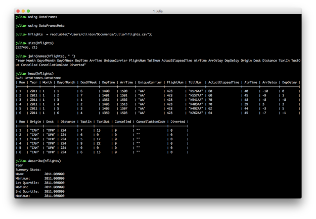
The semicolon on the end of the readtable command prevents it from printing the dataset to the screen. The size command returns the number of rows and columns in the dataset. You can specify you only want the number of rows with size(hflights, 1) or columns with size(hflights, 2). This dataset contains 227,496 rows and 21 columns. The names command lists the column headings. By default, the head command prints the header row and six data rows. You can specify the number of data rows to display by adding a second argument, e.g. head(hflights, 10). The describe command prints summary statistics for each column.
@where: Keep rows matching criteria
AND: All of the conditions must be true for the returned rows
# Julia DataFrames approach to view all flights on January 1

hflights[.&(hflights[:Month] .== 1, hflights[:DayofMonth] .== 1), :]
# DataFramesMeta approach

@where(hflights, :Month .== 1, :DayofMonth .== 1)
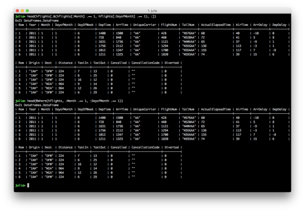
Julia’s DataFrames’ row filtering syntax is similar to R’s syntax. To specify multiple AND conditions, use “.&()” and place the filtering conditions, separated by commas, between the parentheses. Like dplyr’s filter function, DataFramesMeta’s @where macro simplifies the syntax and makes the command easier to read.
OR: One of the conditions must be true for the returned rows
# Julia DataFrames approach to view all flights where either AA or UA is the carrier

hflights[.|(hflights[:UniqueCarrier] .== "AA", hflights[:UniqueCarrier] .== "UA"), :]
# DataFramesMeta approach

@where(hflights, .|(:UniqueCarrier .== "AA", :UniqueCarrier .== "UA"))
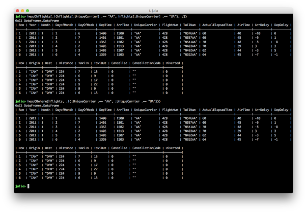
To specify multiple OR conditions, use “.|()” and place the filtering conditions between the parentheses. Again, the DataFramesMeta approach is more concise.
SET: The values in a column are in a set of interest
# Julia DataFrames approach to view all flights where the carrier is in Set(["AA", "UA"])

carriers_set = Set(["AA", "UA"])

hflights[findin(hflights[:UniqueCarrier], carriers_set), :]
# DataFramesMeta approach

@where(hflights, findin(:UniqueCarrier, carriers_set))
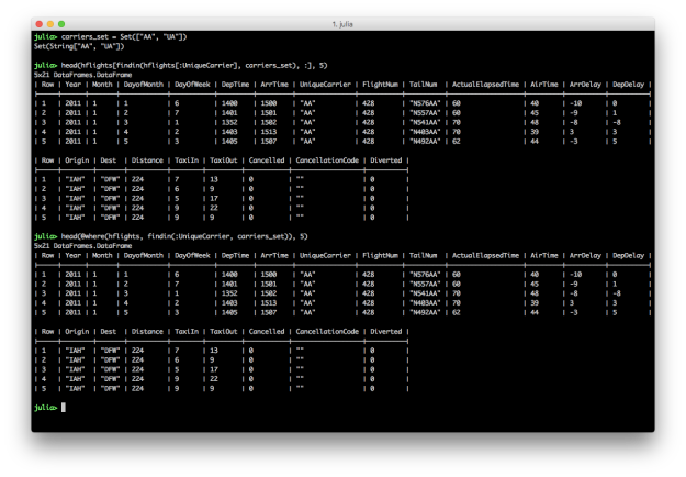
To filter for rows where the values in a particular column are in a specific set of interest, create a Set with the values you’re interested in and then specify the column and your set of interest in the findin function.
PATTERN / REGULAR EXPRESSION: The values in a column match a pattern
# Julia DataFrames approach to view all flights where the carrier matches the regular expression r"AA|UA"

carriers_pattern = r"AA|UA"

hflights[[ismatch(carriers_pattern, String(carrier)) for carrier in hflights[:UniqueCarrier]], :]
# DataFramesMeta approach

@where(hflights, [ismatch(carriers_pattern, String(carrier)) for carrier in :UniqueCarrier])
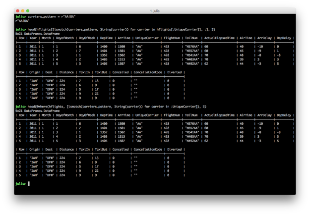
To filter for rows where the values in a particular column match a pattern, create a regular expression and then use it in the ismatch function in an array comprehension.
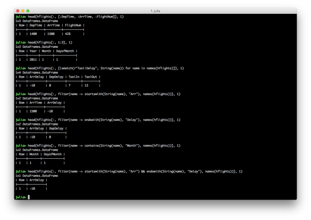
@select: Pick columns by name
# Julia DataFrames approach to selecting columns

hflights[:, [:DepTime, :ArrTime, :FlightNum]]
# DataFramesMeta approach

@select(hflights, :DepTime, :ArrTime, :FlightNum)
Julia’s DataFrames’ syntax for selecting columns is similar to R’s syntax. Like dplyr’s select function, DataFramesMeta’s @select macro simplifies the syntax and makes the command easier to read.
# Julia DataFrames approach to selecting columns

# first three columns

hflights[:, 1:3]

# pattern / regular expression

heading_pattern = r"Taxi|Delay"

hflights[:, [ismatch(heading_pattern, String(name)) for name in names(hflights)]]

# startswith

hflights[:, filter(name -> startswith(String(name), "Arr"), names(hflights))]

# endswith

hflights[:, filter(name -> endswith(String(name), "Delay"), names(hflights))]

# contains

hflights[:, filter(name -> contains(String(name), "Month"), names(hflights))]
# AND conditions

hflights[:, filter(name -> startswith(String(name), "Arr") && endswith(String(name), "Delay"), names(hflights))]

# OR conditions

hflights[:, filter(name -> startswith(String(name), "Arr") || contains(String(name), "Cancel"), names(hflights))]
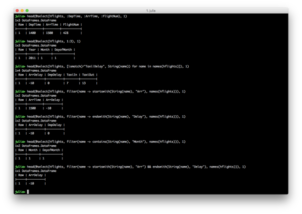
# DataFramesMeta approach

# first three columns

@select(hflights, 1:3)

# pattern / regular expression

heading_pattern = r"Taxi|Delay"

@select(hflights, [ismatch(heading_pattern, String(name)) for name in names(hflights)])

# startswith

@select(hflights, filter(name -> startswith(String(name), "Arr"), names(hflights)))

# endswith

@select(hflights, filter(name -> endswith(String(name), "Delay"), names(hflights)))

# contains

@select(hflights, filter(name -> contains(String(name), "Month"), names(hflights)))
# AND conditions

@select(hflights, filter(name -> startswith(String(name), "Arr") && endswith(String(name), "Delay"), names(hflights)))

# OR conditions

@select(hflights, filter(name -> startswith(String(name), "Arr") || contains(String(name), "Cancel"), names(hflights)))
# Kevin Markham's multiple select conditions example

# select(flights, Year:DayofMonth, contains("Taxi"), contains("Delay"))

# Julia Version of Kevin's Example

# Taxi or Delay in column heading

mask = [ismatch(r"Taxi|Delay", String(name)) for name in names(hflights)]

# Also include first three columns, i.e. Year, Month, DayofMonth

mask[1:3] = true

@select(hflights, mask)
These examples show you can select columns by position and name, and you can combine multiple conditions with AND, “&&”, or OR, “||”. Similar to filtering rows, you can select specific columns based on a pattern by using the ismatch function in an array comprehension. You can also use contains, startswith, and endswith in the filter function to select columns that contain, start with, or end with a specific text pattern.
“Chaining” or “Pipelining”
In R, dplyr provides, via the magrittr package, the %>% operator, which enables you to chain together multiple commands into a single data transformation pipeline in a very readable fashion. In Julia, the DataFramesMeta package provides the @linq macro and |> symbol to enable similar functionality. Alternatively, you can load the Lazy package and use an @> begin end block to chain together multiple commands.
# Chaining commands with DataFrameMeta’s @linq macro

@linq hflights[find(.!isna.(hflights[:,:DepDelay])), :] |>

@where(:DepDelay .> 60) |>

@select(:UniqueCarrier, :DepDelay)
# Chaining commands with Lazy’s @> begin end block

using Lazy

@> begin

hflights[find(.!isna.(hflights[:,:DepDelay])), :]

@where(:DepDelay .> 60)

@select(:UniqueCarrier, :DepDelay)

end
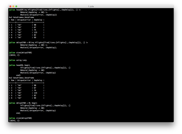
These two blocks of code produce the same result, a DataFrame containing carrier names and departure delays for which the departure delay is greater than 60. In each chain, the first expression is the input DataFrame, e.g. hflights. In these examples, I use the find and !isna. functions to start with a DataFrame that doesn’t contain NA values in the DepDelay column because the commands fail when NAs are present. I prefer the @linq macro version over the @> begin end version because it’s so similar to the dplyr-magrittr syntax, but both versions are more succinct and readable than their non-chained versions. The screen shot shows how to assign the pipeline results to variables.
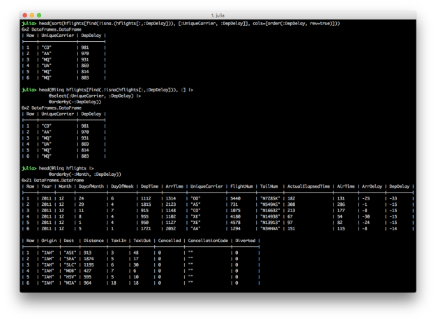
@orderby: Reorder rows
Both DataFrames and DataFramesMeta provide functions for sorting rows in a DataFrame by values in one or more columns. In the first pair of examples, we want to select the UniqueCarrier and DepDelay columns and then sort the results by the values in the DepDelay column in descending order. The last example shows how to sort by multiple columns with the @orderby macro.
# Julia DataFrames approach to sorting

sort(hflights[find(.!isna.(hflights[:,:DepDelay])), [:UniqueCarrier, :DepDelay]], cols=[order(:DepDelay, rev=true)])
# DataFramesMeta approach (add a minus sign before the column symbol for descending)

@linq hflights[find(.!isna.(hflights[:,:DepDelay])), :] |>

@select(:UniqueCarrier, :DepDelay) |>

@orderby(-:DepDelay)
# Sort hflights dataset by Month, descending, and then by DepDelay, ascending

@linq hflights |>

@orderby(-:Month, :DepDelay)
DataFrames provides the sort and sort! functions for ordering rows in a DataFrame. sort! orders the rows, inplace. The DataFrames user guide provides additional examples of ordering rows, in ascending and descending order, based on multiple columns, as well as applying functions to columns, e.g. uppercase, before using the column for sorting.
DataFramesMeta provides the @orderby macro for ordering rows in a DataFrame. Specify multiple column names in the @orderby macro to sort the rows by multiple columns. Use a minus sign before a column name to sort in descending order.
@transform: Add new variables
Creating new variables in Julia DataFrames is similar to creating new variables in Python and R. You specify a new column name in square brackets after the name of the DataFrame and assign it a collection of values, sometimes based on values in other columns. DataFramesMeta’s @transform macro simplifies the syntax and makes the transformation more readable.
# Julia DataFrames approach to creating new variable

hflights[:Speed] = hflights[:Distance] ./ hflights[:AirTime] .* 60

hflights[:, [:Distance, :AirTime, :Speed]]
# Delete the variable so we can recreate it with DataFramesMeta approach

delete!(hflights, :Speed)
# DataFramesMeta approach

@linq hflights |>

@select(:Distance, :AirTime) |>

@transform(Speed = :Distance ./ :AirTime .* 60) |>

@select(:Distance, :AirTime, :Speed)
# Save the new column in the original DataFrame

hflights = @linq hflights |>

@transform(Speed = :Distance ./ :AirTime .* 60)
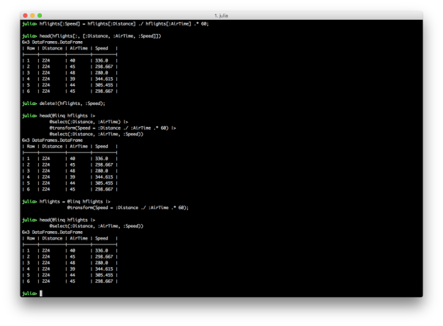
The first code block illustrates how to create a new column in a DataFrame and assign it values based on values in other columns. The second code block shows you can use delete! to delete a column. The third example demonstrates the DataFramesMeta approach to creating a new column using the @transform macro. The last example shows how to save a new column in an existing DataFrame using the @transform macro by assigning the result of the transformation to the existing DataFrame.
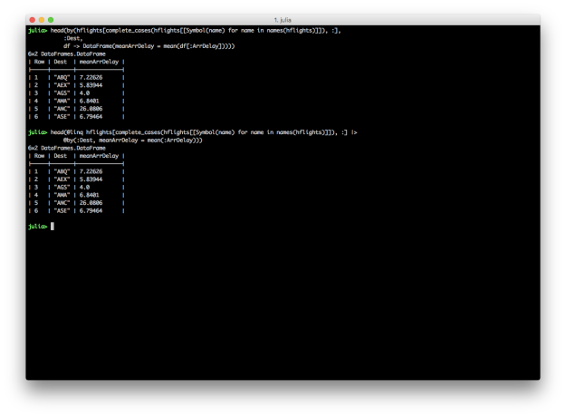
@by: Reduce variables to values (Grouping and Summarizing)
dplyr provides group_by and summarise functions for grouping and summarising data. DataFrames and DataFramesMeta also support the split-apply-combine strategy with the by function and the @by macro, respectively. Here Julia versions of Kevin’s summarise examples.
# Julia DataFrames approach to grouping and summarizing

by(hflights[complete_cases(hflights[[Symbol(name) for name in names(hflights)]]), :],

:Dest,

df -> DataFrame(meanArrDelay = mean(df[:ArrDelay])))
# DataFramesMeta approach

@linq hflights[complete_cases(hflights[[Symbol(name) for name in names(hflights)]]), :] |>

@by(:Dest, meanArrDelay = mean(:ArrDelay))
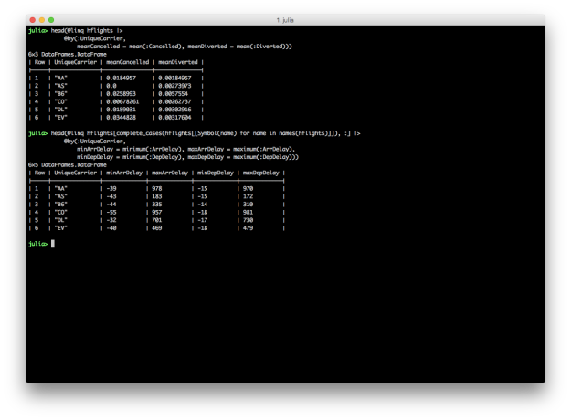
DataFrames and DataFramesMeta don’t have dplyr’s summarise_each function, but it’s easy to apply different functions to multiple columns inside the @by macro.
@linq hflights |>

@by(:UniqueCarrier,

meanCancelled = mean(:Cancelled), meanDiverted = mean(:Diverted))
@linq hflights[complete_cases(hflights[[Symbol(name) for name in names(hflights)]]), :] |>

@by(:UniqueCarrier,

minArrDelay = minimum(:ArrDelay), maxArrDelay = maximum(:ArrDelay),

minDepDelay = minimum(:DepDelay), maxDepDelay = maximum(:DepDelay))
DataFrames and DataFramesMeta also don’t have dplyr’s n and n_distinct functions, but you can count the number of rows in a group with size(df, 1) or nrow(df), and you can count the number of distinct values in a group with countmap.
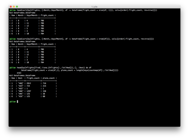
# Group by Month and DayofMonth, count the number of flights, and sort descending

# Count the number of rows with size(df, 1)

sort(by(hflights, [:Month,:DayofMonth], df -> DataFrame(flight_count = size(df, 1))), cols=[order(:flight_count, rev=true)])
# Group by Month and DayofMonth, count the number of flights, and sort descending

# Count the number of rows with nrow(df)

sort(by(hflights, [:Month,:DayofMonth], df -> DataFrame(flight_count = nrow(df))), cols=[order(:flight_count, rev=true)])
# Split grouping and sorting into two separate operations

g = by(hflights, [:Month,:DayofMonth], df -> DataFrame(flight_count = nrow(df)))

sort(g, cols=[order(:flight_count, rev=true)])
# For each destination, count the total number of flights and the number of distinct planes

by(hflights[find(.!isna.(hflights[:,:TailNum])),:], :Dest) do df

DataFrame(flight_count = size(df,1), plane_count = length(keys(countmap(df[:,:TailNum]))))

end
While these examples reproduce the results in Kevin’s dplyr tutorial, they’re definitely not as succinct and readable as the dplyr versions. Grouping by multiple columns, summarizing with counts and distinct counts, and gracefully chaining these operations are areas where DataFrames and DataFramesMeta can improve.
Other useful convenience functions
Randomly sampling a fixed number or fraction of rows from a DataFrame can be a helpful operation. dplyr offers the sample_n and sample_frac functions to perform these operations. In Julia, StatsBase provides the sample function, which you can repurpose to achieve similar results.
using StatsBase

# randomly sample a fixed number of rows

hflights[sample(1:nrow(hflights), 5), :]

hflights[sample(1:size(hflights,1), 5), :]
# randomly sample a fraction of rows

hflights[sample(1:nrow(hflights), ceil(Int,0.0001*nrow(hflights))), :]

hflights[sample(1:size(hflights,1), ceil(Int,0.0001*size(hflights,1))), :]
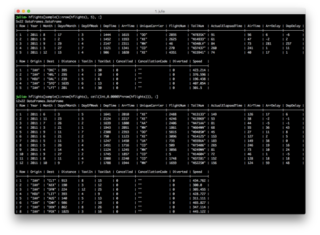
Randomly sampling a fixed number of rows is fairly straightforward. You use the sample function to randomly select a fixed number of rows, in this case five, from the DataFrame. Randomly sampling a fraction of rows is slightly more complicated because, since the sample function takes an integer for the number of rows to return, you need to use the ceil function to convert the fraction of rows, in this case 0.0001*nrow(hflights), into an integer.
Conclusion
In R, dplyr sets a high bar for wrangling data well with succinct, readable code. In Julia, DataFrames and DataFramesMeta provide many useful functions and macros that produce similar results; however, some of the syntax isn’t as concise and clear as it is with dplyr, e.g. selecting columns in different ways and chaining together grouping and summarizing operations. These are areas where Julia’s packages can improve.
I enjoyed becoming more familiar with Julia by reproducing much of Kevin’s dplyr tutorial. It was also informative to see differences in functionality and readability between dplyr and Julia’s packages. I hope you enjoyed this tutorial and find it to be a useful reference for wrangling data in Julia.
Filed under: Analytics, General, Julia, Python, R, Statistics Tagged: DataFrames, DataFramesMeta, dplyr, Julia, Python, R 
![]()


