By: Picaud Vincent
Re-posted from: https://pixorblog.wordpress.com/2016/06/27/some-remarks-about-minmax-functions/
Computing the min (or max) of two values looks like a trivial task.
For C++ the default Standard Template Library implementation is
inline const _Tp& min(const _Tp& __a, const _Tp& __b)
{
    return __b < __a ? __b : __a;
}
However for numerical computations this definition does not mix well with the IEEE 754 standard when dealing with potential NaN value.
For instance, min() is not commutative and is not equivatent to cmath::fmin().
We have:
#include <iostream>
#include <cmath>
#include <limits>
#include <cassert>

using namespace std;

int main()
{
    const auto x_nan = numeric_limits<double>::quiet_NaN();
    const auto x_1 = 1.;

    cout << boolalpha;

    cout << "\n\ncommutativity?";

    cout << "\n min: "
     << (min(x_1, x_nan) == min(x_nan, x_1));

    cout << "\nfmin: "
     << (fmin(x_1, x_nan) == fmin(x_nan, x_1));
}
commutativity?
 min: false
fmin: true
The IEEE 754 says:
In section 6.2 of the revised IEEE 754-2008 standard there are two anomalous functions (the maxnum and minnum functions that return the maximum of two operands that are expected to be numbers) that favor numbers — if just one of the operands is a NaN then the value of the other operand is returned.
On the opposite you can read about C++ rules here:
NaN values have the curious property that they compare as “unordered” with all values, even with themselves. In other words, if x is a NaN, and y is any floating-point value, NaN or not, then x<y, x>y, x<=y, x>=y, and x==y are all false, and x!=y is true.
Remark In C/C++ that is the reason why you can implement the isnan function by
bool isnan(const double x) { return x!=x;}
Using min/max in numerical code
C++
Like the IEEE 754 and C++ standard do not mix well, I personally redefine min()/max() functions as follow:
#include <type_traits>
#include <cmath>

namespace libraryNamespace
{
    template <typename T>
    inline enable_if_t<is_floating_point<T>::value, T>
      min(const T& t1, const T& t2)
    {
        return fmin(t1, t2);
    }

    template <typename T>
    constexpr enable_if_t<is_integral<T>::value, const T&>
      min(const T& t1, const T& t2)
    {
        return (t1 < t2) ? t1 : t2;
    }
    // max() function follows the same scheme
}
Julia
Julia follows the scheme I use in C++, you have a specialization for floating point numbers julia/base/math.jl
min{T<:AbstractFloat}(x::T, y::T) =
    ifelse((y < x) | (signbit(y) > signbit(x)),
           ifelse(isnan(y), x, y), ifelse(isnan(x), y, x))
and a generic operator julia/base/operator.jl
min(x,y) = ifelse(y < x, y, x)
We can check that the Float specialization follows the IEEE 754 rule:
(max(5,NaN)==max(NaN,5))&&(max(5,NaN)==5)
true
What is the cost?
Julia
There is a big difference between the simple definition in julia/base/operator.jl and the NaN aware code of julia/base/math.jl.
We can have a look at the assembly code.
I would like to thank Erik Schnetter who made me noticed that Julia 4.6 @code_native was bugged (see his comment at the end of this post). Hence to get the same result you must have a recent Julia version. In this post I use:
versioninfo()
Julia Version 0.5.0-dev+5453
Commit 1fd440e (2016-07-15 23:33 UTC)
Platform Info:
  System: Linux (x86_64-linux-gnu)
  CPU: Intel(R) Core(TM) i3 CPU       M 380  @ 2.53GHz
  WORD_SIZE: 64
  BLAS: libopenblas (USE64BITINT DYNAMIC_ARCH NO_AFFINITY Nehalem)
  LAPACK: libopenblas64_
  LIBM: libopenlibm
  LLVM: libLLVM-3.7.1 (ORCJIT, westmere)
With this Julia version you get the following asm codes:
@code_native(min(1,2))
gives
	.text
Filename: promotion.jl
	pushq	%rbp
	movq	%rsp, %rbp
Source line: 257
	cmpq	%rdi, %rsi
	cmovgeq	%rdi, %rsi
	movq	%rsi, %rax
	popq	%rbp
	retq
whereas
@code_native min(1.0,2.0)
gives
	.text
Filename: math.jl
	pushq	%rbp
	movq	%rsp, %rbp
Source line: 203
	ucomisd	%xmm1, %xmm0
	seta	%al
	movmskpd	%xmm1, %ecx
	movmskpd	%xmm0, %edx
	andl	$1, %edx
	xorb	$1, %dl
	andb	%cl, %dl
	orb	%al, %dl
	je	L54
	movapd	%xmm1, %xmm2
	cmpordsd	%xmm2, %xmm2
	andpd	%xmm2, %xmm1
	andnpd	%xmm0, %xmm2
	orpd	%xmm1, %xmm2
	jmp	L75
L54:
	movapd	%xmm0, %xmm2
	cmpordsd	%xmm2, %xmm2
	andpd	%xmm2, %xmm0
	andnpd	%xmm1, %xmm2
	orpd	%xmm0, %xmm2
L75:
	movapd	%xmm2, %xmm0
	popq	%rbp
	retq
	nopw	%cs:(%rax,%rax)
C++
We have the same in C++
#include <cmath>
#include <iostream>

int main()
{
  double x, y;
  std::cin >> x >> y;
  asm("#ASM FOR FMIN");
  double fmin_x_y = std::fmin(x, y);
  asm("#ASM FOR FMIN - END");
  std::cout << "\n" << fmin_x_y;

  asm("#ASM FOR MIN");
  double min_x_y = std::min(x, y);
  asm("#ASM FOR MIN - END");
  std::cout << "\n" << min_x_y;
  return 0;
}
compiled with
g++ -std=c++11 -O3 -S min.cpp -o min.asm
gives for min()
#ASM FOR MIN
	movsd	24(%rsp), %xmm0
	minsd	16(%rsp), %xmm0
	movsd	%xmm0, 8(%rsp)
#ASM FOR MIN - END
and for fmin()
#ASM FOR FMIN
	movsd	24(%rsp), %xmm1
	movsd	16(%rsp), %xmm0
	call	fmin
	movsd	%xmm0, 8(%rsp)
#ASM FOR FMIN - END
CPU time?
Illustration with the Jaccard distance defined by

We compute this distance using 4 different approaches:
- Julia min()/max() NaN aware
- Julia min()/max() comparison
- C fmin()/fmax() NaN aware
- C min()/max() comparison
The Julia code is given below
function jaccard_julia_NaN_aware(a::Array{Float64,1},
                                 b::Array{Float64,1})

    @assert length(a)==length(b)

    num::Float64 = 0
    den::Float64 = 0

    for i in 1:length(a)

        @inbounds num += min(a[i],b[i])
        @inbounds den += max(a[i],b[i])

    end
    return 1. - num/den
end

function jaccard_julia_comparison(a::Array{Float64,1},
                                  b::Array{Float64,1})

    @assert length(a)==length(b)

    num::Float64 = 0
    den::Float64 = 0

    for i in 1:length(a)

        @inbounds num += ifelse(a[i]<b[i],a[i],b[i])
        @inbounds den += ifelse(a[i]>b[i],a[i],b[i])

    end
    return 1. - num/den
end

function jaccard_C_NaN_aware(a::Array{Float64,1},
                             b::Array{Float64,1})

    @assert length(a)==length(b)

    return ccall((:jaccard_C_NaN_aware,
                  "./libjaccard.so"),
                 Float64,
                 (Int64,Ptr{Float64},Ptr{Float64}),
                 length(a),a,b)

end

function jaccard_C_comparison(a::Array{Float64,1},
                              b::Array{Float64,1})

    @assert length(a)==length(b)

    return ccall((:jaccard_C_comparison,
                  "./libjaccard.so"),
                 Float64,
                 (Int64,Ptr{Float64},Ptr{Float64}),
                 length(a),a,b)

end

function test_distance(f,
                       v1::Array{Float64,1},
                       v2::Array{Float64,1})
    sum=0
    for i in 1:5000
        sum+=f(v1,v2)
    end
    sum
end

v1=rand(10000);
v2=rand(10000);

for name in (:jaccard_julia_NaN_aware,
             :jaccard_C_NaN_aware,
             :jaccard_julia_comparison,
             :jaccard_C_comparison)
    print("$name")
    @time @eval test_distance($name,v1,v2)
end
The associated C subroutines are:
#include <math.h>
#include <stdint.h>

double jaccard_C_NaN_aware(uint64_t size,
               double *a, double *b)
{
  double num = 0, den = 0;

  for(uint64_t i = 0; i < size; ++i)
    {
      num += fmin(a[i],b[i]);
      den += fmax(a[i],b[i]);
    }
  return 1. - num / den;
}

double jaccard_C_comparison(uint64_t size,
                double *a, double *b)
{
  double num = 0, den = 0;

  for(uint64_t i = 0; i < size; ++i)
    {
      num += (a[i] < b[i] ? a[i] : b[i]);
      den += (a[i] > b[i] ? a[i] : b[i]);
    }
  return 1. - num / den;
}
and the Makefile is
all: bench

bench: libjaccard.so
    @julia --optimize --check-bounds=no jaccard.jl

libjaccard.so: jaccard.c
    @gcc -O2 -shared -fPIC jaccard.c -o libjaccard.so
The results I get on my computer are:
make
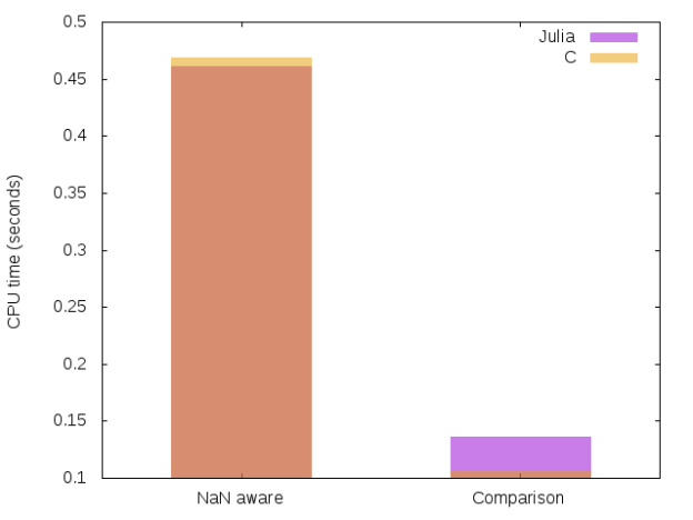
We see that:
- for the NaN aware case C and Julia running time is equivalent, great!
- for the Comparison case C seems to be a little bit faster, but the gap is very small and more precise benchmark would be necessary to quantify it.
- min()/max() using simple comparisons is more than 3.5 times faster than an implementation taking into account possible NaN values.
Julia 4.6 previous results
In the first version of this post, using julia version 4.6, I got this result:
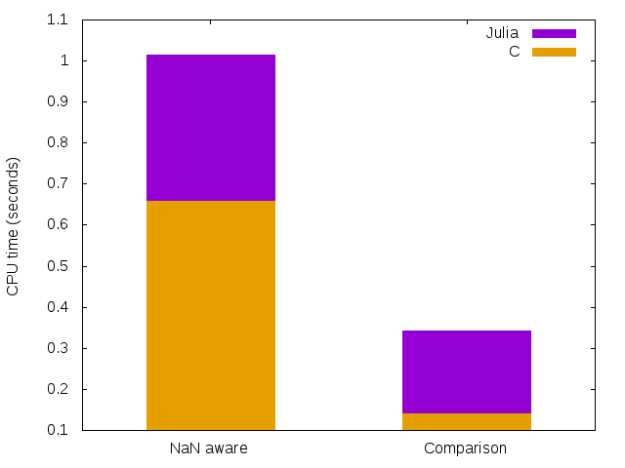
There was a clear advantage for the C code, but it seems this is not the case anymore with julia version 0.5.
You can reproduce the results of this post, using the code available on GitHub.
A source of bugs?
You have to take care that a simple statement like

is mathematically true but false in your code. It is even false for both the IEEE 754 and the comparison based versions of the min() function.
In the future I will write a post on Automatic Differentiation. To be brief automatic differentiation is a tool that allows you to efficiently compute gradient with nearly no modification of your original code. As example my personal implementation takes the form:
// Declare the current tape
//
AD_Tape<double> tape;

// Computes gradient of f(x,y,z)=x.z.sin(x.y)
//                   at (x,y,z)=(2,1,5)
//
// Note:
//
// grad(f)={ x * y * z * Cos(x * y) + z * Sin(x * y),
//           x^2 * z *
//           Cos(x * y), x * Sin(x * y) }
//
AD_Scalar<double> x, y, z, f;

x = 2;
y = 1;
z = 5;

f = x * z * sin(x * y);

const auto grad = ad_gradient(f);

std::cout << "\ngrad(f) = {"
          << grad[x] << ","
          << grad[y] << ","
          << grad[z] << "}";

// The screen output is
//
// grad(f) = {0.385019,-8.32294,1.81859}
One classical approach uses operator overloading. For each basic operation you compute the function value and its differential.
One important and desirable property of AutoDiff library is that its use does not modify your program result.
Unfortunately a lot of AutoDiff libraries are bugged when they define the min()/max() functions.
It is really “natural” to define min() overloading by something like:
function min(x,y)
    ifelse(x<y,
           return (x,dx),
           return (y,dy))
But this implementation is buggy: if y is NaN we now know that x<y is always false, hence:
- the original code will return x
- the AutoDiff code will return (y,dy) (a priori =(NaN,NaN))
To stay consistent the correct implementation is something like:
function min(x,y)
    ifelse(x==min(x,y),
           return (x,dx),
           return (y,dy))
which provides the right result (id consistent with the original code) whatever x or y is NaN or not
We can check that, for instance, with Julia ForwardDiff.jl
(githash: 045a828)
using ForwardDiff
f(x::Vector)=max(2*x[1],x[2]);
x=[1.,NaN]
print("Original value: $(f(x))")
print("\nAutoDiff gradient: $(ForwardDiff.gradient(f, x))")
Original value: 2.0
AutoDiff gradient: [0.0,1.0]
which is wrong, in this case the right gradient is
![\nabla [(x_1,x_2)\rightarrow max(2.x_1,x_2)]_{x_1=1,x_2=NaN}=(2,0)](https://s0.wp.com/latex.php?latex=%5Cnabla+%5B%28x_1%2Cx_2%29%5Crightarrow+max%282.x_1%2Cx_2%29%5D_%7Bx_1%3D1%2Cx_2%3DNaN%7D%3D%282%2C0%29+&bg=ffffff&%23038;fg=1a1a1a&%23038;s=0 "\nabla [(x_1,x_2)\rightarrow max(2.x_1,x_2)]_{x_1=1,x_2=NaN}=(2,0)")
Final word
-
Concerning min()/max() examples of this post I have observed a big performance gain in using Julia version 5.0. What is not clear is the reason of this gain:
- I compiled my own version of Julia 5.0, but I used the 4.6 version shipped with Debian. Maybe my compiled version uses some different compiler flags (like -march=native
 ).
). - or there is a real improvement between version 4.6 -> 5.0
You can reproduce the benchmark using the code available on GitHub. Any feed back is welcome.
- I compiled my own version of Julia 5.0, but I used the 4.6 version shipped with Debian. Maybe my compiled version uses some different compiler flags (like -march=native
- The @native_code macro of Julia version 4.6 seems to be bugged.
- It is “easy” to introduce bugs when you mix comparison operators and IEEE 754 min()/max() functions. Implementing min()/max() in a Automatic Differentiation framework is one perfect illustration of this and was the point that motivated me to write this post.
- (Joke) If you are fed up with min()/max() you can use absolute value:


but these relations do not follow the IEEE 754 standard!
I would like to thank my colleague JP. Both for having noticed that min()/max() was “abnormally” slow (Julia 4.6), Y. Borstein for some emails exchanges concerning min()/max() in Julia (before I wrote this post), Erik Schnetter who told me to switch to a more recent Julia version.