Author Archives: Dean Markwick's Blog -- Julia

Benchmarking maps, loops, generators and broadcasting in Julia

By: Dean Markwick's Blog -- Julia

Re-posted from: https://dm13450.github.io/2019/05/03/Map-Loop-Generator.html

A few weeks ago I wrote a blog post about the speed differences
between map and loop. I posted it to reddit and got some feedback
on a) why the map was so slow and b) other ways the calculation
could be made which are just as quick as a loop. In this post I’m
writing about these new methods and adding them to the comparison.


Enjoy these types of posts? Then sign up for my newsletter.


Previous Methods

For a more detailed explanation of the problem I’m trying to solve, check out my previous
post
here. For
now I’m just going to recap.

using BenchmarkTools
using Statistics
clusterLabels = [1,1,2,2,3,3,5]

We started off with a simple map.

function pointsPerCluster_map(clusterLabels)
    map(i-> sum(clusterLabels .== i), 1:maximum(clusterLabels))
end

pointsPerCluster_map(clusterLabels)

mapBM = @benchmark pointsPerCluster_map($clusterLabels)
BenchmarkTools.Trial: 
  memory estimate:  21.73 KiB
  allocs estimate:  18
  --------------
  minimum time:     2.944 μs (0.00% GC)
  median time:      3.624 μs (0.00% GC)
  mean time:        7.479 μs (44.30% GC)
  maximum time:     9.851 ms (99.91% GC)
  --------------
  samples:          10000
  evals/sample:     8

It turns out this was slow because with each call of the function I
was creating a temporary array with clusterLabels .== i. To improve
on this I wrote the loop explicitly.

function pointsPerCluster_loop(clusterLabels)

    maxSize = maximum(clusterLabels)
    ppc = zeros(Int64, maxSize)
    
    for i in clusterLabels
        ppc[i] += 1
    end
    ppc
end
pointsPerCluster_loop(clusterLabels)

loopBM = @benchmark pointsPerCluster_loop($clusterLabels)
BenchmarkTools.Trial: 
  memory estimate:  128 bytes
  allocs estimate:  1
  --------------
  minimum time:     53.756 ns (0.00% GC)
  median time:      82.478 ns (0.00% GC)
  mean time:        167.708 ns (21.97% GC)
  maximum time:     240.429 μs (99.95% GC)
  --------------
  samples:          10000
  evals/sample:     985

The loop method was the easy winner and orders of magnitudes
quicker. But now we’ve got some new methods to test.

New Methods

The first two methods are from a reddit comment
here. The
final new method is taken from the Performance Tips section of the
Julia documentation.

Generator

First off, we use a generator. This is a better map implementation as
it doesn’t create the temporary array, instead it runs a tally of how
many entries are equal to i for each i we are mapping across.

function pointsPerCluster_gen(clusterLabels)
    map(i-> sum(c == i for c in clusterLabels), 1:maximum(clusterLabels))
    
end

pointsPerCluster_gen(clusterLabels)

genBM = @benchmark pointsPerCluster_gen($clusterLabels)
BenchmarkTools.Trial: 
  memory estimate:  336 bytes
  allocs estimate:  8
  --------------
  minimum time:     128.594 ns (0.00% GC)
  median time:      135.287 ns (0.00% GC)
  mean time:        203.392 ns (26.73% GC)
  maximum time:     131.934 μs (99.77% GC)
  --------------
  samples:          10000
  evals/sample:     891

The results are in the nanosecond range, which is great, same order
of magnitude as the loop.

Broadcasting .

In Julia, to apply a function to each element in a vector you use .
after the function which easy vectorisation. For example sin.(x)
will apply sine to each element of x. Whereas sin(x) would error.
In this case we can create an anonymous function that applies to each
element of our array.

pointsPerCluster_broad(clusterLabels) = (k->mapreduce(i->i==k, +, clusterLabels)).(1:maximum(clusterLabels))

pointsPerCluster_broad(clusterLabels)

broadBM = @benchmark pointsPerCluster_broad($clusterLabels)
BenchmarkTools.Trial: 
  memory estimate:  128 bytes
  allocs estimate:  1
  --------------
  minimum time:     96.824 ns (0.00% GC)
  median time:      101.509 ns (0.00% GC)
  mean time:        136.465 ns (13.67% GC)
  maximum time:     94.869 μs (99.85% GC)
  --------------
  samples:          10000
  evals/sample:     947

Again, the average speed is in the nanosecond range so comparable to
the loop.

Inbounds Loop

Another method of improving performance that the official
documentation recommends (with warning) is the @simd macro and the
@inbounds macro. These are compiler level optimisations that turn
off some of the safety features in the name of speed. With the caveat
that misbehaviour of the function could be catastrophic. We decorate
the loop function with these macros and test the results.

function pointsPerCluster_loop_inb(clusterLabels)

    maxSize = maximum(clusterLabels)
    ppc = zeros(Int64, maxSize)
    
    @simd for i in clusterLabels
        @inbounds ppc[i] += 1
    end
    ppc
end
pointsPerCluster_loop_inb(clusterLabels)

inboundsBM = @benchmark pointsPerCluster_loop_inb($clusterLabels)
BenchmarkTools.Trial: 
  memory estimate:  128 bytes
  allocs estimate:  1
  --------------
  minimum time:     51.369 ns (0.00% GC)
  median time:      56.292 ns (0.00% GC)
  mean time:        80.677 ns (24.89% GC)
  maximum time:     87.980 μs (99.89% GC)
  --------------
  samples:          10000
  evals/sample:     986

Again on the nanosecond scale, so all is working well.

Visualising

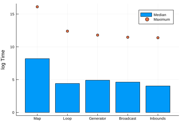
You know what this post needs: graphs. Here we plot the median and
maximum time the benchmarking tool reports.

using Plots
nms = ["Map", "Loop", "Generator", "Broadcast"]
bmList = [mapBM, loopBM ,genBM, broadBM]

timeArray = mapreduce(x -> [minimum(x).time, median(x).time, maximum(x).time], hcat, bmList)'
bar(nms, log.(timeArray[:, 2]), seriestype=:scatter, labels="Median", yaxis=("log Time"))
plot!(nms, log.(timeArray[:, 3]), seriestype=:scatter, labels="Maximum")
Log running times

bar(nms[2:4], (timeArray[2:4, 2]), seriestype=:scatter, yaxis=("Time"), label="Median")

We have to plot the \(\log\) of the running times as the naive map
is that much slower. The other methods are all about the same though,
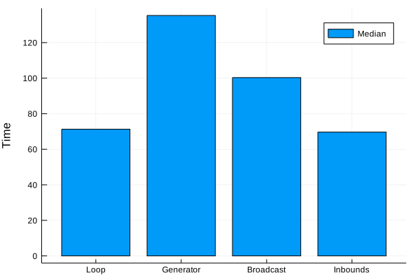
so lets remove the map and focus on the fast methods.
Median running times

Here we can see that the loop method is still the fastest. The methods
provided in the feedback improve on the naive map but still cannot
compete with the loop. Using the @simd and @inbounds macro don’t change the overall median
value for it to be worth the potential danger.

Overall there are lots of ways to accomplish this task, but the loop
still comes out on top. Even using the “go-faster” macros doesn’t
improve on the runtime significantly.
Speed differences between a map and a loop in Julia

By: Dean Markwick's Blog -- Julia

Re-posted from: https://dm13450.github.io/2019/04/17/MapLoopPerformance.html

I’m currently writing some of my R functions in Julia to improve
performance. In R it is bad form to write a loop. Instead there are
functions like lapply and vapply that map a function across a
list. They are much faster and can be more readable than writing a
loop. So in converting the code to Julia I was replacing the lapply
functions to map. Then I would benchmark the Julia function compared
to the R function and I was seeing a performance benefit but nothing
to write home about. This was troubling as the
benchmarks suggest that Julia is
much faster than R. I was doing something wrong and decided to
investigate the performance difference between a loop and map in
Julia.

using BenchmarkTools
using Statistics

In this simple example, we want to count the amount of elements are
assigned a cluster label.

clusterLabels = [1,1,2,2,3,3,5]

The naive implementation using map can be written as:

function pointsPerCluster_map(clusterLabels)
    map(i-> sum(clusterLabels .== i), 1:maximum(clusterLabels))
end

pointsPerCluster(clusterLabels)

mapBM = @benchmark pointsPerCluster_map($clusterLabels)
BenchmarkTools.Trial: 
  memory estimate:  21.73 KiB
  allocs estimate:  18
  --------------
  minimum time:     2.794 μs (0.00% GC)
  median time:      4.319 μs (0.00% GC)
  mean time:        6.917 μs (41.06% GC)
  maximum time:     6.618 ms (99.87% GC)
  --------------
  samples:          10000
  evals/sample:     8

So of the order of microseconds, which seems reasonable enough. When
you write the same code in R you get a median of about 6-7
microseconds. So the Julia gets about a 2x speed up, nice!

But when you unpack the map and write it in a loop the results are
almost unbelievable.

function pointsPerCluster_loop(clusterLabels)

    maxSize = maximum(clusterLabels)
    ppc = zeros(Int64, maxSize)
    
    for i in clusterLabels
        ppc[i] += 1
    end
    ppc
end
pointsPerCluster_loop(clusterLabels)

loopBM = @benchmark pointsPerCluster_loop($clusterLabels)
BenchmarkTools.Trial: 
  memory estimate:  128 bytes
  allocs estimate:  1
  --------------
  minimum time:     53.101 ns (0.00% GC)
  median time:      57.738 ns (0.00% GC)
  mean time:        91.857 ns (13.29% GC)
  maximum time:     57.285 μs (99.79% GC)
  --------------
  samples:          10000
  evals/sample:     985

By using a for loop we are now in nanosecond territory. We can
extract the median runtime of both approaches and use the judge
function to give a final say.

judge(median(mapBM), median(loopBM))
BenchmarkTools.TrialJudgement: 
  time:   +7380.62% => regression (5.00% tolerance)
  memory: +17287.50% => regression (1.00% tolerance)

A performance improvement of 7,000% and 17,000% better memory performance. Unbelievable results!

If you are making the leap from R to Julia like for like
translation might not be optimal. Instead start thinking about loops again

Which Turing.jl Sampler is the Fastest?

By: Dean Markwick's Blog -- Julia

Re-posted from: https://dm13450.github.io/2019/04/10/Turing-Sampling-Speed.html

The Turing.jl package provides a great interface
for performing Bayesian inference using a variety of algorithms. But
what algorithm allows you to go from data to samples the quickest? In
this blog post I will be sampling from a simple model to demonstrate
how quickly you can sample from a model. This is useful
for anyone that has a Turing model in the middle of another model that
they need to get samples from.

Toy Model

For the toy model we will be sampling from the Beta distribution.

using Distributions

testData = rand(Beta(3, 4), 100);

Writing the model in Julia is simple enough. We will be using an
inverse Gamma prior for the free parameters.

using Turing
Turing.turnprogress(false)

@model betaSample(y) = begin
    
    alpha ~ InverseGamma(2, 1/8)
    beta ~ InverseGamma(2, 1/8)
    
    for i in eachindex(y)
        y[i] ~ Beta(alpha, beta)
    end
	end
	
sample(betaSample(testData), MH(250))
[MH] Finished with
  Running time        = 0.6196572280000009;
  Accept rate         = 0.028;

Object of type Chains, with data of type 250×4×1 Array{Union{Missing, Float64},3}

Log evidence      = 0.0
Iterations        = 1:250
Thinning interval = 1
Chains            = 1
Samples per chain = 250
internals         = elapsed, lp
parameters        = alpha, beta

parameters
       Mean    SD   Naive SE  MCSE    ESS 
alpha 0.4483 0.1063   0.0067 0.0453 5.4955
 beta 0.2394 0.0461   0.0029 0.0191 5.8285

This quick test verifies that I’ve written the model correctly and everything can be sampled.

Available Samplers

In this blog post I am interested in being able to quickly sample from the posterior distribution and extract some sensible parameter samples. I will be assessing 4 different samplers.

  • Hamiltonian Monte Carlo (HMC)
  • Metropolis Hastings (MH)
  • No U Turn Sampling (NUTS)
  • Stochastic Gradient Langevin Dynamics (SGLD)

Each have their own way of sampling from the posterior distribution,
with benefits and drawbacks. Turing provides an standard interface to
use these algorithms without having to worry about the fine details.

We want to be able to ‘set and forget’ the parameters of the sampler
so will be using the defaults given at
http://turing.ml/docs/sampler-viz/. If the sampling fails, I will
tweak the parameters until it works.

I’ve chosen these 4 samplers out of familiarity. HMC and NUTS are the
algorithms used in Stan. Metropolis Hastings is the one sampler
everyone has implemented themselves at one point and SGLD is an
improved version of that. I’m not including the particle samplers,
mainly because I’m unfamiliar with their use cases.

We will be running the samplers for 1000 iterations and benchmarking for 120 seconds. This should give us enough trials to calculate an average running time of the samplers.

using BenchmarkTools
BenchmarkTools.DEFAULT_PARAMETERS.seconds = 120.0

numIts = 1000

HMC

hmcSamps = sample(betaSample(testData), HMC(numIts, 0.01, 10));
hmcRunTime = @benchmark sample(betaSample($testData), HMC($numIts, 0.01, 10));

Metropolis Hastings

mhSamps = sample(betaSample(testData), MH(numIts));
mhRunTime = @benchmark sample(betaSample($testData), MH($numIts));

NUTS

nutsSamps = sample(betaSample(testData), NUTS(numIts, 0.65));
nutsRunTime = @benchmark sample(betaSample($testData), NUTS($numIts, 0.65));

SGLD

sgldSamps = sample(betaSample(testData), SGLD(numIts, 0.01));
sgldRunTime = @benchmark sample(betaSample($testData), SGLD($numIts, 0.01));

Results

using Plots
function extractMeanTime(runtime)
    median(runtime).time /1e9 
end

nms = ["SGLD", "HMC", "MH", "NUTS"]
runTimes = [sgldRunTime, hmcRunTime, mhRunTime, nutsRunTime]

times = map(extractMeanTime, runTimes)

map(length, runTimes)
4-element Array{Int64,1}:
 340
  38
 287
  23

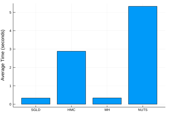
Here we can see that each sampler has been evaluated a number of times. The median running time is extracted and converted into seconds.

bar(nms, times, ylabel="Average Time (seconds)", legend=false)

svg

HMC and NUTS are the slowest. SGLD and MH performing the
quickest which is the expected result. The calculations involved in
the HMC and NUTS algorithms are a bit more complex.

However, it is not always about speed. We want to make sure that the
sampler is moving towards the correct parameters and not just moving
about randomly. We need to a check the quality of the samples. To assess this we want to check the Effective Number
of Samples
which is a metric that discounts the samples by the
autocorrelation between values. Essentially, a better sampling
algorithm will produce a higher number of effective samples for the
same number of iterations.

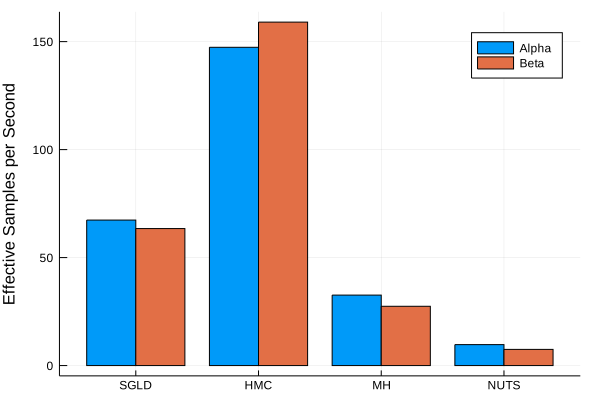
Therefore, instead of just looking at the running time, we want to
divide the effective sample size by the running time to produce a
Effective Samples per Second value.

function extractMeanandESS(smps)
    params = MCMCChains.summarystats(smps)
    alphaESS = params.summaries[1].value[1, 5,1]
    betaESS = params.summaries[1].value[2, 5,1]
    
    alphaMean = params.summaries[1].value[1, 1,1]
    betaMean = params.summaries[1].value[2, 1,1]
    
    [alphaMean, betaMean, alphaESS, betaESS]
end

allSamps = [sgldSamps, hmcSamps, mhSamps, nutsSamps]
params = map(extractMeanandESS, allSamps)
paramSummaries = reduce(hcat, params)'
4×4 LinearAlgebra.Adjoint{Float64,Array{Float64,2}}:
 2.6097  3.1185   22.4958   21.1824
 2.8535  3.3886  424.781   458.39  
 0.3993  0.7389   11.0827    9.3238
 2.9507  3.5326   51.6685   39.9213
using StatsPlots
alphaESSperSecond = paramSummaries[:,3] ./ times
betaESSperSecond = paramSummaries[:,4] ./ times

groupedbar(nms, hcat(alphaESSperSecond, betaESSperSecond), label=["Alpha", "Beta"], ylabel="Effective Samples per Second")

svg

So NUTS produces the least amount of effective samples per second run. Which is surprising, but for such a simple model it doesn’t cause too much of a concern. I would predict that as the model increased in complexity, the ESS would improve compared to the other samplers.

From this graph, we are inclined to think that either HMC or SGLD are the preferable sampling algorithms.

Parameter Results

pdfs = map(x-> pdf.(Beta(x[1], x[2]), collect(0:0.01:1)), params)

histogram(testData, normed=true, label="Training Data", fillalpha=0.4)

plot!(collect(0:0.01:1), pdfs[1], label=nms[1], linewidth=2)
plot!(collect(0:0.01:1), pdfs[2], label=nms[2], linewidth=2)
plot!(collect(0:0.01:1), pdfs[3], label=nms[3], linewidth=2)
plot!(collect(0:0.01:1), pdfs[4], label=nms[4], linewidth=2)
plot!(collect(0:0.01:1), pdf.(Beta(3,4), collect(0:0.01:1)), label="True", linewidth=2)

svg

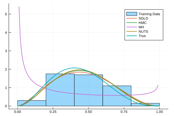
Here we can see that the Metropolis Hastings sampler is nowhere near the true distribution. All the others have done well and are close to the true distribution. Given that they only have 100 datapoints to go by and we are just taking the mean of the samples its not a bad result.

Conclusion

So in conclusion it looks like we would be inclined to use the HMC
sampler. It produces the best ESS per second values and doesn’t
require too much tinkering with. If speed is an absolute priority,
then SGLD might be more appropriate, its 6 times faster at the cost of
about 100 effective samples a second.

Definitely do not use Metropolis Hastings though. Out of the box it hasn’t even got close to the correct value. I’m probably missing setting some parameter.

There are a number of weaknesses in this analysis. Firstly, we have not considered multiple chains to check for convergence. Currently, multiple chains in parallel are not supported out of the box for Turing.jl so rather than faff about using multiple chains by hand, I’ve just stuck to the one. Secondly, BenchmarkTools runs for a fixed amount of time rather than a fixed amount of samples. I’ve changed the parameters of the benchmark to try and account for this, but it still isn’t exact.
Finally, there are still the particle samplers. I’ve shied away from
them, mainly because I’ve never used them before and not 100% on their
use case.