Author Archives: Dean Markwick's Blog -- Julia

Julia Code for Sampling an AR(1) model

By: Dean Markwick's Blog -- Julia

Re-posted from: https://dm13450.github.io/2017/06/12/Auto-Julia.html

In my previous blog post I outlined the basic AR(1) model and the necessary maths needed to infer the unknown parameter \(\phi\). In this post I will outline some basic Julia code to build a MCMC sampler for such a model to infer the unknown parameter \(\phi\).

Firstly, we need to simulate some data. From the previous post we know that the data \(y\) comes simply from the previous value, plus some fixed noise. In Julia this is simply writing a for loop and using the Distributions package to sample some white noise.

function simulate_ar(phi, n)

	 dist = Normal()

	 y = [0.0 for i = 1:n]

	 noise = rand(dist, n)

	 for i in 1:(n-1)

	     y[i+1] = phi*y[i] + noise[i] 
	 end

	 return y
end

For 1000 data points with \(\phi=0.5\) such a process looks like:
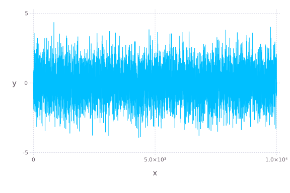
AR1 Process Plot

Pretty much looks like a random walk around 0 as expected.

Now to compute the statistics for the posterior distribution we need
the sum of squares and the lagged sum of squares ( [see here] (https://dm13450.github.io/2017/06/09/Bayesian-Auto-Process.html)). Then using the Distributions package again we can sample from a truncated normal distribution. We have used a prior distribution of a truncated normal distribution with 0 mean and a standard deviation of 5.

function posterior_ar(n, y)
	 n = length(y)
	 ss = sum(y .* y) + 1/25 
	 ss_lagged = sum(y .* vcat(y[2:n],0))
	 
	 dist = Truncated(Normal(ss_lagged/ss, sqrt(1/ss)), -1, 1)
	 smps = rand(dist, n)

	 return smps
end
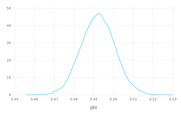
Phi Density Plot

So we can see that the posterior distribution for \(\phi\) is close to the true value of 0.5, so it looks like our algorithm is working.

Although its just a toy model in these posts I have shown how to calculate the posterior for an autoregressive process and how to draw from such a distribution using Julia. Next stop, include more parameters and see how flexible autoregressive models can be.
Bayesian Autoregressive Processes

By: Dean Markwick's Blog -- Julia

Re-posted from: https://dm13450.github.io/2017/06/09/Bayesian-Auto-Process.html

An autoregressive process can be described by the equation

\[y_t = c + \phi y_{t-1} + \epsilon.\]

The parameter \(c\) is some baseline, \(\phi\) if between -1 and 1, and \(\epsilon\) is some white noise process. If we consult the Wikipedia article on such process we find that there it is fairly trivial to calculate the unknown parameter \(\phi\) in a frequentist setting. Googling about for a Bayesian introduction didn’t turn up anything particularly helpful, so here I try to plug that gap.

For any Bayesian method we need to decompose our problem into three parts; likelihood, prior and posterior distribution. For simplicity we will be setting \(c=0\).

For the likelihood we can see that each observation \(y_i\) is normally distributed around \(\phi y_{i-1}\) with variance equal to that of the white noise process \(\epsilon\)

\[p(y_i | y_1, \ldots , y_n , \sigma _\epsilon ^2) \propto \frac{1}{\sigma _\epsilon} \exp \left( \frac{-(y_i – \phi y_{i-1})^2}{2 \sigma _\epsilon ^2} \right),\]

now the likelihood is just this density multiplied across all the data.

Now for the prior. Like any Gaussian inference problem it is a smart choice to use a Gaussian prior on \(\phi\) so that we get a conjugate prior. But there is a hard limit on the values of the parameter in question \(-1 < \phi < 1\), therefore we must use the truncated normal distribution.

\[(\phi | \mu _0 , \sigma _0 ^2) = \frac{\exp \left( – \frac{ (\phi – \mu_0) ^2}{2 \sigma _0 ^2} \right)}{\sqrt{2 \pi} \sigma_0 \left(\Phi \left( \frac{b-\mu_0}{\sigma _0} \right) – \Phi \left( \frac{a-\mu_0}{\sigma _0} \right) \right) }\]

the values of \(a , b\) set the limits of the truncation, so in our case they will be \(-1, 1\) respectively.

So lets combine both the likelihood and the prior to get our posterior distribution for \(\phi\). Due to the conjugacy of the prior, we know that the posterior is also going to be a truncated normal distribution.

\[p( \phi | y_1 , \ldots , y_n, \mu _0 , \sigma _0 ^2, \sigma _{\epsilon} ^2 ) = \text{Truncated-Normal} ( \mu \sigma ^{2 } , \sigma ^2 )\]

\[\mu = \frac{\sum _i y_i y_{i-1}}{\sigma _\epsilon ^2} + \frac{\mu _0}{ \sigma _0 ^2}\]

\[\sigma ^{2 } = \left( \frac{\sum_i y_i ^2}{\sigma _\epsilon ^2} + \frac{1}{\sigma _0^2} \right)^{-1}\]

Now these are simple enough to implement in a few lines of R and with such a simple model I’ll leave that as an exercise to the reader.

References

https://arxiv.org/ftp/arxiv/papers/1611/1611.08747.pdf

https://en.wikipedia.org/wiki/Truncated_normal_distribution

https://en.wikipedia.org/wiki/Autoregressive_model

An Introduction to Julia and Distributions

By: Dean Markwick's Blog -- Julia

Re-posted from: https://dm13450.github.io/2017/01/26/Julia-Distributions.html

Julia is a new language on the block aimed at being a suitable mid point between the adaptability of Python and the speed of Matlab. Its a nice fall-back when my R code is just that bit too slow to really churn through some numbers.

On of the main benefits of using R is the ease at which the ‘standard’ distributions are available. Want exponentially distributed random variables? Just call rexp()! Want the pdf of the gamma distribution? dgamma() is there to help you. With Julia this type of functionality is in the Distribution module, so takes just a little bit more of work to get the same functionality.

In this post I will outline how the basics of the distributions package and how you can replicate some of the functionality of R.

Firstly, we need to install the Distributions package. This is done by calling Pkg.add("Distributions"). Now that is installed we need to load it into the namespace. Open a new Julia instance and load the package with using Distributions. The necessary functions are now loaded.

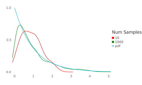
Our first exercise will be to sample \(N\) exponentially distributed variables and check that the density of the samples tends to the pdf of the exponential distribution as \(N\) becomes larger.
The first step in this code is to define our distribution. As the exponential distribution only requires one parameter, \(m\), this is as simple as calling Exponential(m) in our code. Now we use a number of different functions on the distribution.

We can sample from this distribution using rand(dist, N) where \(N\) is the number of samples to draw. We can then overlay the pdf of the distribution by using pdf(dist, x).

Combing these commands allows us to draw a graph (using the Julia package Gadfly) like this:

Exponential Plot

Here we can see the small sample size does not resemble the pdf but the large sample size does. So we are correctly drawing from the exponential distribution as expected.

There are also other functions available. A great example is calculating the mean of a log-normal distribution. This distribution is defined with two parameters; \(m\) and \(s^2\). However, the mean of the distribution is not equal to \(m\). Instead it is \(\exp(m+\frac{s^2}{2})\). The Distributions package in Julia knows this. So by simply calling mean on the LogNormal() object you can return the theoretical mean of the distribution and not have to worry about the parametrisation specifics of the distribution.

dist = LogNormal(1,4)
mean(dist) == exp(1 + 4^2/2)

Overall, Julia and the Distributions package offer similar functionality to R. You can easily replicate some of the functions in R with very effort in Julia. This can be a useful tool if R is not quite cutting it on the speed front.