By: Dean Markwick's Blog -- Julia

Re-posted from: https://dm13450.github.io/2020/07/05/AlphaVantage.html

AlphaVantage is a market data provider that is nice enough to provide
free access to a wide variety of data. It is my goto financial data
provider ( State of the Market – Infinite State Hidden Markov Models ) , because a) it’s free and b) there is an R package that
accesses the API easily. However, there was no Julia package for
AlphaVantage, so I saw a gap in the market.

After searching GitHub I found the AlphaVantage.jl repository that was two years out
of date, but had the bare bones of functionality that I knew I would
be able to build upon. I forked the project, brought it up to date
with all the AlphaVantage functions and have now released it to the
world in the Julia registry. You can easily install the package just
like any other Julia package using Pkg.add("AlphaVantage").

Enjoy these types of posts? Then you should sign up for my newsletter. It’s a short monthly recap of anything and everything I’ve found interesting recently plus
any posts I’ve written. So sign up and stay informed!

This blog post will detail all the different function available and
illustrate how you can pull the data, massage it into a nice format
and plot using the typical Julia tools.

Available Functionality from AlphaVantage

1. Stock data at both intraday, daily, weekly and monthly
   frequencies.
2. Technical indicators for stocks.
3. FX rates at both intraday, daily, weekly and monthly frequencies.
4. Crypto currencies, again, at the intraday, daily, weekly and monthly
   time scales.

So jump into the section that interests you.

The package is designed to replicate the API functions from the
AlphaVantage documentation,
so you can look up any of the functions there and find the
equivalent in this Julia package. If I’ve missed any or one isn’t
working correctly, raise on issue on Github
here.

These are the Julia packages I use in this blog post:

using AlphaVantage
using DataFrames
using DataFramesMeta
using Dates
using Plots

Plus we define some helper functions to convert between the raw
data and Julia dataframes.

function raw_to_dataframe(rawData)
    df = DataFrame(rawData[1])
    dfNames = Symbol.(vcat(rawData[2]...))
    df = rename(df, dfNames)

    df.Date = Date.(df.timestamp)
    for x in (:open, :high, :low, :close, :adjusted_close, :dividend_amount)
        df[!, x] = Float64.(df[!, x])
    end 
    df.volume = Int64.(df.volume)
    return df
end

function intra_to_dataframe(rawData)
    df = DataFrame(rawData[1])
    dfNames = Symbol.(vcat(rawData[2]...))
    df = rename(df, dfNames)

    df.DateTime = DateTime.(df.timestamp, "yyyy-mm-dd HH:MM:SS")
    for x in (:open, :high, :low, :close)
        df[!, x] = Float64.(df[!, x])
    end 
    df.volume = Int64.(df.volume)
    return df
end

Stock Market Data

AlphaVantage provides daily, weekly and monthly historical stock data from 2000 right up to when you call the function. With the adjusted functions you also get dividends and adjusted closing prices to account for these dividends.

tslaRaw = AlphaVantage.time_series_daily_adjusted("TSLA", outputsize="full", datatype="csv")
tsla = raw_to_dataframe(tslaRaw);
first(tsla, 5)

5 rows × 10 columns (omitted printing of 2 columns)

plot(tsla.Date, tsla.open, label="Open", title="TSLA Daily")

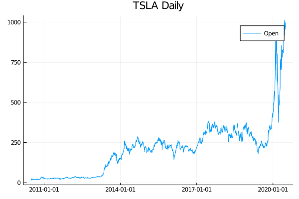
Here is the Tesla daily opening stock price.

Intraday Stock Data

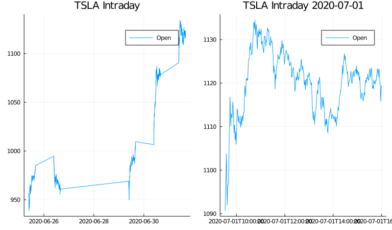
What separates AlphaVantage from say google or yahoo finance data is the intraday data. They provide high frequency bars at intervals from 1 minute to an hour. The only disadvantage is that the maximum amount of data appears to be 5 days for a stock. Still better than nothing!

tslaIntraRaw = AlphaVantage.time_series_intraday("TSLA", "1min", outputsize="full", datatype="csv");
tslaIntra = intra_to_dataframe(tslaIntraRaw)
tslaIntraDay = @where(tslaIntra, :DateTime .> DateTime(today()-Day(1)))
subPlot = plot(tslaIntraDay.DateTime, tslaIntraDay.open, label="Open", title="TSLA Intraday $(today()-Day(1))")
allPlot = plot(tslaIntra.DateTime, tslaIntra.open, label="Open", title = "TSLA Intraday")
plot(allPlot, subPlot, layout=(1,2))

Stock Technical Indicators

AlphaVantage also provide a wide range of technical indicators, the
most of which I don’t understand and will probably never use. But,
they provide them, so I’ve written an interface for them. In this
example I’m using the Relative Strength Index.

rsiRaw = AlphaVantage.RSI("TSLA", "1min", 10, "open", datatype="csv");
rsiDF = DataFrame(rsiRaw[1])
rsiDF = rename(rsiDF, Symbol.(vcat(rsiRaw[2]...)))
rsiDF.time = DateTime.(rsiDF.time, "yyyy-mm-dd HH:MM:SS")
rsiDF.RSI = Float64.(rsiDF.RSI);

rsiSub = @where(rsiDF, :time .> DateTime(today() - Day(1)));
plot(rsiSub[!, :time], rsiSub[!, :RSI], title="TSLA")
hline!([30, 70], label=["Oversold", "Overbought"])

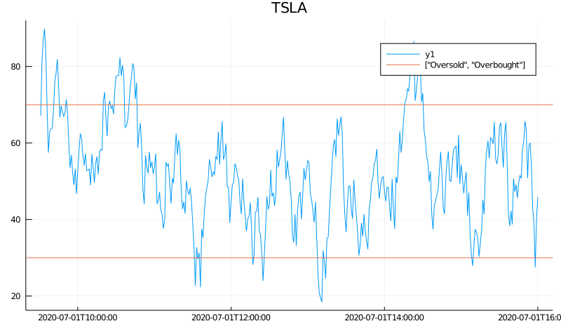
In this case, adding the threshold lines make a nice channel that the value falls between.

Sector Performance

AlphaVantage also provides the sector performance on a number of timescales through one API call.

sectorRaw = AlphaVantage.sector_performance()
sectorRaw["Rank F: Year-to-Date (YTD) Performance"]

Dict{String,Any} with 11 entries:
  "Health Care"            => "-3.46%"
  "Financials"             => "-25.78%"
  "Consumer Discretionary" => "4.79%"
  "Materials"              => "-9.33%"
  "Consumer Staples"       => "-7.80%"
  "Energy"                 => "-38.38%"
  "Real Estate"            => "-11.37%"
  "Information Technology" => "12.06%"
  "Utilities"              => "-12.96%"
  "Communication Services" => "-2.26%"
  "Industrials"            => "-16.05%"

Great year for IT, not so great for energy.

Forex Market Data

Moving onto the foreign exchange market, again, AlphaVantage provide multiple time scales and many currencies.

eurgbpRaw = AlphaVantage.fx_weekly("EUR", "GBP", datatype="csv");
eurgbp = DataFrame(eurgbpRaw[1])
eurgbp = rename(eurgbp, Symbol.(vcat(eurgbpRaw[2]...)))
eurgbp.Date = Date.(eurgbp.timestamp)
eurgbp.open = Float64.(eurgbp.open)
eurgbp.high = Float64.(eurgbp.high)
eurgbp.low = Float64.(eurgbp.low)
eurgbp.close = Float64.(eurgbp.close)
plot(eurgbp.Date, eurgbp.open, label="open", title="EURGBP")

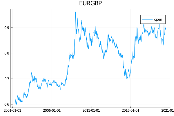
Which looks great for a liquid currency like EURGBP, but they have a whole host of currencies so don’t limit yourself to just the basics, explore some NDF’s.

usdkrwRaw = AlphaVantage.fx_monthly("USD", "KRW", datatype="csv");
usdkrw = DataFrame(usdkrwRaw[1])
usdkrw = rename(usdkrw, Symbol.(vcat(usdkrwRaw[2]...)))
usdkrw.Date = Date.(usdkrw.timestamp)
usdkrw.open = Float64.(usdkrw.open)
usdkrw.high = Float64.(usdkrw.high)
usdkrw.low = Float64.(usdkrw.low)
usdkrw.close = Float64.(usdkrw.close)
plot(usdkrw.Date, usdkrw.open, label="open", title="USDKRW")

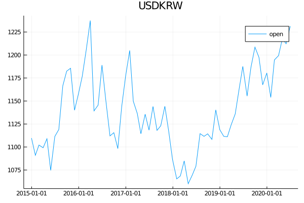
Although I’m not sure exactly what they are providing here, be it a
spot price or a 1 month forward that is more typical for NDFs.

FX Intraday Data

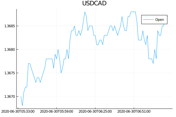
Again, intraday data is available for the FX pairs.

usdcadRaw = AlphaVantage.fx_intraday("USD", "CAD", datatype="csv");
usdcad = DataFrame(usdcadRaw[1])
usdcad = rename(usdcad, Symbol.(vcat(usdcadRaw[2]...)))
usdcad.timestamp = DateTime.(usdcad.timestamp, "yyyy-mm-dd HH:MM:SS")
usdcad.open = Float64.(usdcad.open)
plot(usdcad.timestamp, usdcad.open, label="Open", title="USDCAD")

Crypto Market Data

Now for digital currencies. The API follows the same style as traditional currencies and again has more digital currencies than you can shake a stick at. Again daily, weekly and monthly data is available plus a ‘health-index’ monitor that reports how healthy a cryptocurrency is based on different features.

ethRaw = AlphaVantage.digital_currency_daily("ETH", "USD", datatype="csv")
ethHealth = AlphaVantage.crypto_rating("ETH");
titleString = ethHealth["Crypto Rating (FCAS)"]

Dict{String,Any} with 9 entries:
  "7. utility score"         => "972"
  "9. timezone"              => "UTC"
  "1. symbol"                => "ETH"
  "2. name"                  => "Ethereum"
  "4. fcas score"            => "957"
  "5. developer score"       => "964"
  "6. market maturity score" => "843"
  "8. last refreshed"        => "2020-06-29 00:00:00"
  "3. fcas rating"           => "Superb"

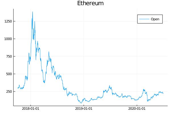
The health rating looks like that, four scores, a qualitative rating
and some meta information. The price charts look like as you would expect.

eth = DataFrame(ethRaw[1])
eth = rename(eth, Symbol.(vcat(ethRaw[2]...)), makeunique=true)
eth.Date = Date.(eth.timestamp)
eth.Open = Float64.(eth[!, Symbol("open (USD)")])

plot(eth.Date, eth.Open, label="Open", title = "Ethereum")

Conclusion

If you’ve ever wanted to explore financial timeseries you can’t really
do much better than using AlphaVantage. So go grab yourself an API
key, download this package and see if you can work out what Hilbert
transform, dominant cycle phase (HT_DCPHASE in the package) represents for a stock!

Be sure to checkout my other tutorials for AlphaVantage:

• Fundamental Stock Data from AlphaVantage.jl
• Crypto Data using AlphaVantatge.jl
• Economic Indicators from AlphaVantage

By: Dean Markwick's Blog -- Julia

Re-posted from: https://dm13450.github.io/2020/05/26/HawkesProcessesPackage.html

HawkesProcesses.jl is a Julia package that provides a number of
functions to model events using a Hawkes process. This vignette
demonstrates how you can use the package and fit Hawkes processes to
your data. Here are the fine details on the
Hawkes process maths.

So download the package and you can follow along with my post.

using HawkesProcesses
using Distributions
using Plots

Enjoy these types of posts? Then sign up for my newsletter.

Intensity of a Hawkes Process

bg = 0.5
kappa = 0.5
kernel(x) = pdf.(Distributions.Exponential(1/0.5), x)
maxT = 100;

We calculate the intensity of a Hawkes process with default parameters all equal to 0.5 between 0 and 10 with two events at t = 3 and 6.

ts = 0:0.1:10
testEvents = [3, 6]
intensity = HawkesProcesses.intensity(collect(ts), testEvents, bg, kappa, kernel);

plot(ts, intensity, xlabel = "Time", ylabel = "Intensity", label="")

As expected two spikes of intensity when the events occur.

Simulating a Hawkes Process

simevents = HawkesProcesses.simulate(bg, kappa, kernel, maxT);

We now simulate events with default parameters from t=0 to t=100.

ts = collect(0:0.1:maxT)
intensity = HawkesProcesses.intensity(ts, simevents, bg, kappa, kernel)
plot(ts, intensity, xlabel="Time", ylabel = "Intensity", label="")
plot!(simevents, repeat([mean(intensity)], length(simevents)), seriestype=:scatter, label="Events")

Again, spikes of events occurring followed by slightly quieter periods which shows the clustering effect of the Hawkes process.

Bayesian Estimation of a Hawkes Processs using a Latent Variable

This package provides an enhanced method of MCMC sampling of the Hawkes process parameters. By exploiting a latent variable (mathematical details can be found here) we are able to more efficiently sample from the posterior distribution than by doing direct Gibbs sampling using the likelihood and prior.

bg = 0.5
kappa = 0.5
kernel(x) = pdf.(Distributions.Exponential(1/0.5), x)
maxT = 1000
simevents = HawkesProcesses.simulate(bg, kappa, kernel, maxT);

bgSamps, kappaSamps, kernSamps = HawkesProcesses.fit(simevents, maxT, 1000);

plot(histogram(bgSamps, label="Background", colour=:darkred), 
    histogram(kappaSamps, label="Kappa", colour=:darkblue), 
    histogram(kernSamps, label="Kernel", colour=:darkgreen), layout = (1, 3))

The histograms of the parameter samples are distributed around the true values as expected which shows our method is working. We run another chain to check convergence.

bgSamps2, kappaSamps2, kernSamps2 = HawkesProcesses.fit(simevents, maxT, 1000);

bgplot = plot(bgSamps, label="Chain 1", title="Background")
bgplot = plot!(bgplot, bgSamps2, label="Chain 2")

kappaplot = plot(kappaSamps, label="Chain 1", title="Kappa")
kappaplot = plot!(kappaSamps2, label="Chain 2")

kernplot = plot(kernSamps, label="Chain 1", title="Kernel")
kernplot = plot!(kernSamps2, label="Chain 2")

plot(bgplot, kappaplot, kernplot, layout = (1, 3))

A basic visual inspection shows that the chains are exploring the parameter space nicely.

Hawkes Process Likelihood

The likelihood of a Hawkes process can be used in a number of ways. It can assess the goodness of fit of a particular parameter set or it can be used to estimate parameters aswell.

bg = 0.5
kappa = 0.5
kernelDist =  Distributions.Exponential(1/0.5)
kernel_f(x) = pdf.(kernelDist, x)
maxT = 1000
simevents = HawkesProcesses.simulate(bg, kappa, kernel_f, maxT);

trueLikelihood = HawkesProcesses.likelihood(simevents, bg, kappa, kernelDist, maxT)

-963.4283337185043

bgArray = collect(0.1:0.05:1)
bgLikelihood = map(x -> HawkesProcesses.likelihood(simevents, x, kappa, kernelDist, maxT), bgArray)
bgPlot = plot(bgArray, bgLikelihood, xlabel="Parameter Values", ylabel = "Likelihood", label="Background", colour=:darkred);

kappaArray = collect(0.1:0.05:1)
kappaLikelihood = map(x -> HawkesProcesses.likelihood(simevents, bg, x, kernelDist, maxT), kappaArray)
kappaPlot = plot(kappaArray, kappaLikelihood, xlabel="Parameter Values", ylabel = "Likelihood", label="Kappa", colour=:darkblue);

kernArray = collect(0.01:0.01:1)
kernLikelihood = map(x -> HawkesProcesses.likelihood(simevents, bg, kappa, Distributions.Exponential(1/x), maxT), kernArray)
kernPlot = plot(kernArray, kernLikelihood, xlabel="Parameter Values", ylabel = "Likelihood", label="Kernel", colour=:darkgreen);

plot(bgPlot, kappaPlot, kernPlot, layout=(3,1))

Here we demonstrate the shape of the likelihood for the different values in parameters. As expected the likelihood reaches its maximum value at the true values.

Maximum Likelihood Estimation of a Hawkes Process

Using the likelihood function from HawkesProcesses we can use optimisation to find the parameters that produce the maximum values of the likelihood.

using Optim
function exp_mle(params, events, maxT)
    if any(params .< 0)
        return Inf
    end
    
    bg = params[1]
    kappa = params[2]
    kernParam = params[3]
    
    -1*HawkesProcesses.likelihood(events, bg, kappa, Distributions.Exponential(kernParam), maxT)
end

opt = optimize(x->exp_mle(x, simEvents, maxT), rand(3)*10)
Optim.minimizer(opt)

3-element Array{Float64,1}:
 0.5155810722101667 
 0.47205389686884425
 2.8440961890338596 

The parameters are close to the true values but this isn’t always the case. In practise the likelihood function of a Hawkes process is very flat around the maximum and can prove difficult to optimise over.

By: Dean Markwick's Blog -- Julia

Re-posted from: https://dm13450.github.io/2019/09/20/Turing-Update.html

One of the creators of the Turing.jl package messaged me a few weeks ago to ask me to rerun my benchmarking tests of the different samplers because they had made some performance improvements. So here I am, being the independent third party to verify these improvements. I hope I can see them and I don’t want to ruin anyone’s Friday night!

In my last blog post (here) I didn’t actually record what version of Julia or Turing I was using which is a bit annoying. I’m 99% certain I was using Julia 1.1 and looking at the Turing releases I imagine it might have been version 0.6.14. My current version of Turing is 0.6.17, but I think I might have updated it at some point after the original blog post so a bit tricky to tell what was used. My plan for this rerun is to update Julia to 1.2 and Turing to the latest version in the package manager, rerun the notebook and post the results.

So after doing exactly that here are the results.

A stunning improvement and quite frankly I’m seriously impressed. Looking at my previous post, NUTS was the slowest with almost 5 seconds for 1000 iterations. Using the latest version of Turing and you get an average of about 0.4 seconds for 1000 iterations so a 10x speed up. Not bad at all! So well done to the Turing team, really knocked it out the park with these latest updates.

In conclusion it looks like Julia 1.2 and Turing 0.6.23 have resulted in a massive performance update for the package and I’m looking forward to where it goes next.