Re-posted from: http://www.stochasticlifestyle.com/julia-on-the-hpc-with-gpus/
This is a continuous of my previous post on using Julia on the XSEDE Comet HPC. Check that out first for an explanation of the problem. In that problem, we wished to solve for the area of a region where a polynomial was less than 1, which was calculated by code like:
@time res = @sync @parallel (+) for i = imin:dx:imax
  tmp = 0
  isq2 = i*i; isq3 = i*isq2; isq4 = isq2*isq2; isq5 = i*isq4
  isq6 = isq4*isq2; isq7 = i*isq6; isq8 = isq4*isq4
  @simd for j=jmin:dx:jmax
    jsq2 = j*j; jsq3= j*jsq2; jsq4 = jsq2*jsq2;
    jsq5 = j*jsq4; jsq6 = jsq2*jsq4; jsq7 = j*jsq6; jsq8 = jsq4*jsq4
    @inbounds tmp += abs(coefs[1]*(jsq2) + coefs[2]*(jsq3) + coefs[3]*(jsq4) + coefs[4]*(jsq5) + coefs[5]*jsq6 + coefs[6]*jsq7 + coefs[7]*jsq8 + coefs[8]*(i) + coefs[9]*(i)*(jsq2) + coefs[10]*i*jsq3
    + coefs[11]*(i)*(jsq4) + coefs[12]*i*jsq5 + coefs[13]*(i)*(jsq6) + coefs[14]*i*jsq7 + coefs[15]*(isq2) + coefs[16]*(isq2)*(jsq2) + coefs[17]*isq2*jsq3 + coefs[18]*(isq2)*(jsq4) +
    coefs[19]*isq2*jsq5 + coefs[20]*(isq2)*(jsq6) + coefs[21]*(isq3) + coefs[22]*(isq3)*(jsq2) + coefs[23]*isq3*jsq3 + coefs[24]*(isq3)*(jsq4) + coefs[25]*isq3*jsq5 +
    coefs[26]*(isq4) + coefs[27]*(isq4)*(jsq2) + coefs[28]*isq4*jsq3 + coefs[29]*(isq4)*(jsq4) + coefs[30]*(isq5) + coefs[31]*(isq5)*(jsq2) + coefs[32]*isq5*jsq3+ coefs[33]*(isq6) +
    coefs[34]*(isq6)*(jsq2) + coefs[35]*(isq7) + coefs[36]*(isq8))<1
  end
  tmp
end
res = res*((imax-imin)*(jmax-jmin)/(length(imin:dx:imax)*length(jmin:dx:jmax)))
println(res)
Notice that this code is massively parallel: at every point we do something and we just sum the values. This means it’s a perfect problem for the GPU. I am going to show you how to do this.
Getting CUDArt Setup
We will be using the CUDArt.jl package. I first had this working with the CUDA.jl package but was informed that going forward we should be using the CUDArt.jl package. There’s really not much of a difference in my implementation.
To get started, you have to go here and install an appropriate version of CUDA. Note that you have to have an NVIDIA GPU in order to do this. I will be using a GTX970 on one computer (Windows), and a GTX980Ti on another. Comet has a queue with 2x Tesla K80s, but that’s probably overkill and you should try to develop locally first. One you have all of that setup, CUDArt.jl should compile some .ptx files upon first use. If it does, you’re good to go.
CUDArt.jl’s page shows you how to get started. However, I am going to add a little caveat. In reality, this is the objective function in a machine learning problem, and so we wish to be able to recompute this as quickly as possible just by swapping out the coefficient array coefs. Therefore all of the other arrays must persist on the GPU.
Here’s what we’re going to do. To maximize performance on the GPU we will use Float32’s. On most GPUs (all except the Teslas and the Titan Black), the double precision floating point capabilities are SEVERELY gimped in comparison (1/32 the performance…). To do this, we setup our calculations as follows:
## Setup CPU-side parameters
imin = -8
imax = 1
jmin = -3
jmax = 3
@time coefs,powz,poww = getCoefficients(A0,A1,B0,B1,α,β1,β2,β3,β4)
iarr = convert(Vector{Float32},collect(imin:dx:imax))
jarr = convert(Vector{Float32},collect(jmin:dx:jmax))
sizei = length(imin:dx:imax)
sizej = length(jmin:dx:jmax)
cudaCores = 1664;
equalDiv = sizei*sizej÷cudaCores + 1

##GPU Code
CUDArt.init(devices(dev->true)) #Initiate the devices
dev = device(0) #Set the GPU to the first GPU
#Move the arrays over
g_iarr = CudaArray(iarr)
g_jarr = CudaArray(jarr)
g_coefs = CudaArray(coefs)
g_tmp = CudaArray(Int32,cudaCores)
Note that if you have multiple GPUs and don’t know which one is which device, you can use the command CUDArt.name(CUDArt.device_properties(number)). Here I have CUDArt.name(CUDArt.device_properties(0)) return “GeForce GTX 970” and CUDArt.name(CUDArt.device_properties(1)) returns “GeForce GTX 750 Ti”, so I use device(0) to use the 970. Note that at any time you can change the device with this command, but be careful since the CudaArrays are stored on the device that you call them from. If you want to use multiple GPUs, you will also need to split up your arrays.
The CUDA Kernal
Now the last thing I need to do is make my function. To do this, we have to go to C. Here is the Cuda kernal for the calculation:
// filename: integration.cu
// Performs the inner integration loop
extern "C"
{
    __global__ void integration(const float *coefs, const float *iArr, const float *jArr, const int sizei, const int sizej, const int equalDiv, int *tmp)
    {
        int index = threadIdx.x + blockIdx.x * blockDim.x;
        int loopInd;
        float i, j, isq2, isq3, isq4, isq5, isq6, isq7, isq8, jsq2, jsq3, jsq4, jsq5, jsq6, jsq7, jsq8,
        int ans = 0;
        for(loopInd=0;loopInd<equalDiv;loopInd=loopInd+1){
          i = iArr[(index*equalDiv+loopInd)/sizej];
          j = jArr[(index*equalDiv+loopInd)%sizej];
          if(index*equalDiv+loopInd >= sizei*sizej){
            break;
          }
          if((index*equalDiv+loopInd)%sizej==0 || loopInd==0){
            isq2 = i*i;
            isq3 = i*isq2;
            isq4 = isq2*isq2;
            isq5 = i*isq4;
            isq6 = isq4*isq2;
            isq7 = i*isq6;
            isq8 = isq4*isq4;
          }
          jsq2 = j*j;
          jsq3 = j*jsq2;
          jsq4 = jsq2*jsq2;
          jsq5 = j*jsq4;
          jsq6 = jsq2*jsq4;
          jsq7 = j*jsq6;
          jsq8 = jsq4*jsq4;
          /*tmp[index*1878+loopInd]= index*1878+loopInd;*/
		      /* changed to zero indexing */
          ans = ans + (abs(coefs[0]*(jsq2) + coefs[1]*(jsq3) + coefs[2]*(jsq4) + coefs[3]*(jsq5) + coefs[4]*jsq6 + coefs[5]*jsq7 + coefs[6]*jsq8 + coefs[7]*(i) + coefs[8]*(i)*(jsq2) + coefs[9]*i*jsq3 + coefs[10]*(i)*(jsq4) + coefs[11]*i*jsq5 + coefs[12]*(i)*(jsq6) + coefs[13]*i*jsq7 + coefs[14]*(isq2) + coefs[15]*(isq2)*(jsq2) + coefs[16]*isq2*jsq3 + coefs[17]*(isq2)*(jsq4) + coefs[18]*isq2*jsq5 + coefs[19]*(isq2)*(jsq6) + coefs[20]*(isq3) + coefs[21]*(isq3)*(jsq2) + coefs[22]*isq3*jsq3 + coefs[23]*(isq3)*(jsq4) + coefs[24]*isq3*jsq5 + coefs[25]*(isq4) + coefs[26]*(isq4)*(jsq2) + coefs[27]*isq4*jsq3 + coefs[28]*(isq4)*(jsq4) + coefs[29]*(isq5) + coefs[30]*(isq5)*(jsq2) + coefs[31]*isq5*jsq3+ coefs[32]*(isq6) + coefs[33]*(isq6)*(jsq2) + coefs[34]*(isq7) + coefs[35]*(isq8))<1);
        }
        tmp[index] = ans;
    }
}
Okay, that’s not nice looking at all, but it’s the same idea as the Julia script. Let me explain this code a little bit. Our function is integration. It takes in all of the variables and an array tmp which we will save the output to. The first call calculates a unique index for each CUDA core. We then setup our variables. Notice that before that we setup equalDiv to calculate how many calculations each core should do in order to evenly divide the work. Thus we loop over equalDiv times (and check if we go over since this will not necessarily come out perfectly). This means that each CUDA core will calculate the same number of  ‘s. We then use the calculated index and the loop index to get our $i$ and $j$. We index down $j$ first, then go by $i$’s. This means it’s ordered as
  . Notice that we achieve this by doing integer division by the size of the j array (truncation will make it an integer), and we get the $j$ index by moding by the size of the $j$ array. Using these $i$’s and $j$’s, we calculate the inner part of the loop. Notice that the calls to coefs had to be changed because C using 0-based indexing (as opposed to Julia’s 1-based indexing). Note that we can use the abs function from the CUDA math library. All of the CUDA math library functions are available.
[Note that when doing CUDA programming you want to allocate as little memory as possible. This is still on the small side so it worked out to be the optimal code. However, in some cases the non-unraveled version may be better due to the overhead of memory allocation.]
So there’s a template for you to play around with. When all of that is in order, we have to compile the kernal. On Windows with visual studio, I had to find out where cl.exe was (for me it was in Visual Studio 12’s directory) and tell the compiler the location of it. The total command was:
nvcc -ptx integration.cu -ccbin "C:Program Files (x86)Microsoft Visual Studio 12.0VCbin"
On Linux it was simpler:
nvcc -ptx integration.cu
From this you get .ptx files. To use the function in Julia, we then use the following code:
md = CuModule("integrationWin.ptx",false)
integrationFunc = CuFunction(md,"integration")
@time launch(integrationFunc, cudaCores, 64, (g_coefs, g_iarr, g_jarr, sizei,sizej,equalDiv,g_tmp,)); res = sum(to_host(g_tmp));
res = res*((imax-imin)*(jmax-jmin)/(length(imin:dx:imax)*length(jmin:dx:jmax)))
println(res)
What this does is take the “integration” function out of the .ptx and save it as integrationFunc. I can then call it at any time with the launch command. The second and third options are the grid and block sizes. In CUDA you always want to “overload”/overthread the cores so that there is no downtime. What I have found in my tests is that the best setting for this is to set the gridsize to the number of CUDA cores (since in our case these aren’t communicating) and overloading it by setting the block size to 64. Why 64? That worked out best in testing. Change the numbers around and see what works best for you.
The last argument to launch is the tuple of arguments for our integration function. Notice that there is a trailing comma, this is required. After the computation is finished, the results have been saved directly into g_tmp. Thus we send g_tmp to the host and sum up the results as before. We re-scale by the area of integration and that is the result.
Now in the actual objective function, what I want to do is update the coefficients to a new coefficients array, perform this calculation, and then move on. To do this I simply use the code:
    if gpuEnabled
      g_coefs = CudaArray(coefs)
      launch(integrationFunc, cudaCores, 64, (g_coefs, g_iarr, g_jarr, sizei,sizej,equalDiv,g_tmp,))
      res = sum(to_host(g_tmp))
      free(g_coefs)
    else ...
Notice I send coefs over to the GPU, run the kernal to get the answer, and then free up the GPU memory. So in my code I loop over this many times, changing coefs every time. When the entire computation is done, I finish with the command
CUDArt.close(devices(dev->true))
This will clear the GPU.
Comet?
These same steps will work on Comet. You will need to go into an interactive job to compile, but it should work fine. The job script to run Julia on the GPU node is:
#!/bin/bash
#SBATCH -A <account>
#SBATCH --job-name="jOpt"
#SBATCH --output="output/jOpt.%j.%N.out"
#SBATCH -p gpu
#SBATCH --gres=gpu:1
#SBATCH --nodes=1
#SBATCH --export=ALL
#SBATCH --ntasks-per-node=6
#SBATCH -t 48:00:00
export SLURM_NODEFILE=`generate_pbs_nodefile`
/home/crackauc/julia-a2f713dea5/bin/julia --machinefile $SLURM_NODEFILE /home/crackauc/projectCode/ImprovedSRK/Optimization/cometDriver.jl
Here I am only taking 6 nodes for the other computations, and I tell it to use the gpu node with -p and tell it I want only one GPU resource with –gres=gpu:1. If you want to use multiple GPUs, just change that number. However, you will want to split up the arrays amongst the multiple GPUs, change equalDiv to account for each CUDA core doing less calculations, send an integer to the GPU to tell it which GPU it is, and use that integer to change the indexing so that no calculations are repeated. That sounds like a good exercise.
The post Tutorial for Julia on the HPC with GPUs appeared first on Stochastic Lifestyle.


 denote consumption and
  denote leisure. Consider an agent who wishes to maximize Cobb-Douglas utility over consumption and leisure, that is,
 .
. is the relative preference for consumption. The budget constraint is given by,
 ,
, is the wage observed in the data,
  is other income that is not observed in the data, and
  is the tax rate.
 subject to the budget constraint. We assume that non-labor income is uncorrelated with the wage offer, so that
 ![\mathbb{E}[\epsilon_i | w_i]=0](https://s0.wp.com/latex.php?latex=%5Cmathbb%7BE%7D%5B%5Cepsilon_i+%7C+w_i%5D%3D0&bg=ffffff&%23038;fg=333333&%23038;s=0 "\mathbb{E}[\epsilon_i | w_i]=0") . Although this assumption is a bit unrealistic, as we expect high-wage agents to also tend to have higher non-labor income, it helps keep the example simple. The model is also a bit contrived in that we treat the tax rate as unobservable, but this only makes our job more difficult.
. Although this assumption is a bit unrealistic, as we expect high-wage agents to also tend to have higher non-labor income, it helps keep the example simple. The model is also a bit contrived in that we treat the tax rate as unobservable, but this only makes our job more difficult. and
and  and the assumed structure. In particular, the econometrician is interested in the policy-relevant parameter
  , where,
 ,
, denotes the demand for consumption.
  is the marginal propensity for an agent with wage
  is the population average marginal propensity to consume in response to the tax rate. Of course, we can solve the model analytically to find that
  and
and  , where
  is the average wage, but we will show that the numerical methods achieve the correct answer even when we cannot solve the model.

 and
and  that agents in this model would choose. We implement this in Julia as follows:
 ,
,  ,
,  , and
, and  . We draw the wage to have distribution
  , but this is arbitrary.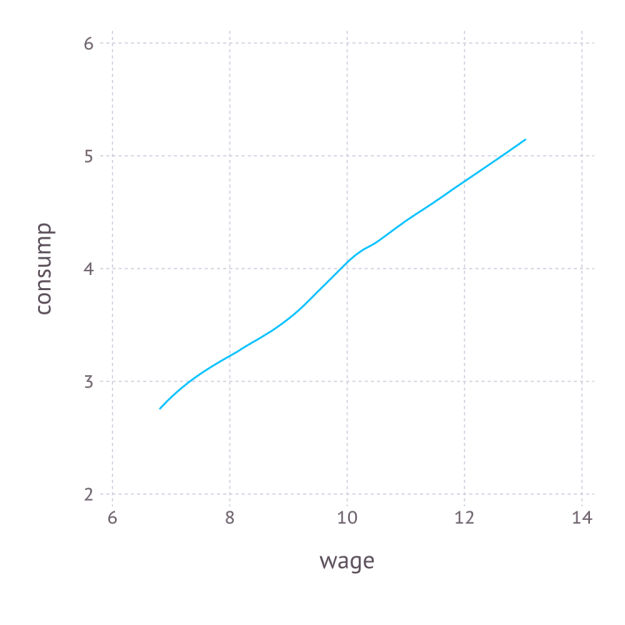
 values of
  :
: for each
  , we have enough information to simulation
  and
and  , for each
  and
and  . With these, we can define the moments,
![\hat{m}\left(\gamma,\tau\right)=\mathbb{E}_{\epsilon}\left[\begin{array}{c} \frac{1}{N}\sum_{i}\left[\hat{c}_{i}\left(\epsilon\right)-c_{i}\right]\\ \frac{1}{N}\sum_{i}\left[\hat{l}_{i}\left(\epsilon\right)-l_{i}\right] \end{array}\right]](https://s0.wp.com/latex.php?latex=%5Chat%7Bm%7D%5Cleft%28%5Cgamma%2C%5Ctau%5Cright%29%3D%5Cmathbb%7BE%7D_%7B%5Cepsilon%7D%5Cleft%5B%5Cbegin%7Barray%7D%7Bc%7D+%5Cfrac%7B1%7D%7BN%7D%5Csum_%7Bi%7D%5Cleft%5B%5Chat%7Bc%7D_%7Bi%7D%5Cleft%28%5Cepsilon%5Cright%29-c_%7Bi%7D%5Cright%5D%5C%5C+%5Cfrac%7B1%7D%7BN%7D%5Csum_%7Bi%7D%5Cleft%5B%5Chat%7Bl%7D_%7Bi%7D%5Cleft%28%5Cepsilon%5Cright%29-l_%7Bi%7D%5Cright%5D+%5Cend%7Barray%7D%5Cright%5D&bg=ffffff&%23038;fg=333333&%23038;s=0 "\hat{m}\left(\gamma,\tau\right)=\mathbb{E}_{\epsilon}\left[\begin{array}{c} \frac{1}{N}\sum_{i}\left[\hat{c}_{i}\left(\epsilon\right)-c_{i}\right]\\ \frac{1}{N}\sum_{i}\left[\hat{l}_{i}\left(\epsilon\right)-l_{i}\right] \end{array}\right]")
![\left(\hat{\gamma},\hat{\tau}\right)=\arg\min_{\gamma\in\left[0,1\right],\tau\in\left[0,1\right]}\hat{m}\left(\gamma,\tau\right)'W\hat{m}\left(\gamma,\tau\right)](https://s0.wp.com/latex.php?latex=%5Cleft%28%5Chat%7B%5Cgamma%7D%2C%5Chat%7B%5Ctau%7D%5Cright%29%3D%5Carg%5Cmin_%7B%5Cgamma%5Cin%5Cleft%5B0%2C1%5Cright%5D%2C%5Ctau%5Cin%5Cleft%5B0%2C1%5Cright%5D%7D%5Chat%7Bm%7D%5Cleft%28%5Cgamma%2C%5Ctau%5Cright%29%27W%5Chat%7Bm%7D%5Cleft%28%5Cgamma%2C%5Ctau%5Cright%29&bg=ffffff&%23038;fg=333333&%23038;s=0 "\left(\hat{\gamma},\hat{\tau}\right)=\arg\min_{\gamma\in\left[0,1\right],\tau\in\left[0,1\right]}\hat{m}\left(\gamma,\tau\right)'W\hat{m}\left(\gamma,\tau\right)")
 is a
is a  weighting matrix, which is only relevant when the number of moments is greater than the number of parameters, which is not true in our case, so
 ![\left(\hat{\gamma},\hat{\tau}\right)=\arg\min_{\gamma\in\left[0,1\right],\tau\in\left[0,1\right]}\left\{ \mathbb{E}_{\epsilon}\left[\frac{1}{N}\sum_{i}\left[\hat{c}_{i}\left(\epsilon\right)-c_{i}\right]\right]\right\} ^{2}+\left\{ \mathbb{E}_{\epsilon}\left[\frac{1}{N}\sum_{i}\left[\hat{l}_{i}\left(\epsilon\right)-l_{i}\right]\right]\right\} ^{2}](https://s0.wp.com/latex.php?latex=%5Cleft%28%5Chat%7B%5Cgamma%7D%2C%5Chat%7B%5Ctau%7D%5Cright%29%3D%5Carg%5Cmin_%7B%5Cgamma%5Cin%5Cleft%5B0%2C1%5Cright%5D%2C%5Ctau%5Cin%5Cleft%5B0%2C1%5Cright%5D%7D%5Cleft%5C%7B+%5Cmathbb%7BE%7D_%7B%5Cepsilon%7D%5Cleft%5B%5Cfrac%7B1%7D%7BN%7D%5Csum_%7Bi%7D%5Cleft%5B%5Chat%7Bc%7D_%7Bi%7D%5Cleft%28%5Cepsilon%5Cright%29-c_%7Bi%7D%5Cright%5D%5Cright%5D%5Cright%5C%7D+%5E%7B2%7D%2B%5Cleft%5C%7B+%5Cmathbb%7BE%7D_%7B%5Cepsilon%7D%5Cleft%5B%5Cfrac%7B1%7D%7BN%7D%5Csum_%7Bi%7D%5Cleft%5B%5Chat%7Bl%7D_%7Bi%7D%5Cleft%28%5Cepsilon%5Cright%29-l_%7Bi%7D%5Cright%5D%5Cright%5D%5Cright%5C%7D+%5E%7B2%7D&bg=ffffff&%23038;fg=333333&%23038;s=0 "\left(\hat{\gamma},\hat{\tau}\right)=\arg\min_{\gamma\in\left[0,1\right],\tau\in\left[0,1\right]}\left\{ \mathbb{E}_{\epsilon}\left[\frac{1}{N}\sum_{i}\left[\hat{c}_{i}\left(\epsilon\right)-c_{i}\right]\right]\right\} ^{2}+\left\{ \mathbb{E}_{\epsilon}\left[\frac{1}{N}\sum_{i}\left[\hat{l}_{i}\left(\epsilon\right)-l_{i}\right]\right]\right\} ^{2}")
 , we need to run sim_moments(params) many times and take the unweighted average across them to achieve the expectation across
  , for some small
  , as follows:
 to be approximately
  on average, while the true value is
  , so the econometrician’s problem is successfully solved.
