An Introduction to Structural Econometrics in Julia

Re-posted from: http://juliaeconomics.com/2016/02/09/an-introduction-to-structural-econometrics-in-julia/

This tutorial is adapted from my Julia introductory lecture taught in the graduate course Practical Computing for Economists, Department of Economics, University of Chicago.

The tutorial is in 5 parts:

Installing Julia + Juno IDE, as well as useful packages
Defining a structural econometric challenge
Data generation, management, and regression visualization
Numerical simulation of optimal agent behavior under constraints
Parallelized estimation by the Method of Simulated Moments

1. Installing Julia + Juno IDE, as well as useful packages

Perhaps the greatest obstacle to using Julia in the past has been the absence of an easy-to-install IDE. There used to be an IDE called Julia Studio which was as easy to use as the popular RStudio for R. Back then, you could install and run Julia + Julia Studio in 5mins, compared to the hours it could take to install Python and its basic packages and IDE. When Julia version 0.3.X was released, Julia Studio no longer worked, and I recommended the IJulia Notebook, which requires the installation of Python and IPython just to use Julia, so any argument that Julia is more convenient to install than Python was lost.

Now, with Julia version 0.4.X, Juno has provided an excellent IDE that comes pre-bundled with Julia for convenience, and you can install Julia + Juno IDE in 5mins. Here are some instructions to help you through the installation process:

Go to http://julialang.org/downloads/ and look for “Julia + Juno IDE bundles“. Click to download the bundle for your system (Windows, Mac, or Linux).
After the brief download (the entire Julia language + Juno IDE is less than 1GB), open the file and click through the installation instructions.
Open Juno, and try to run a very simple line of code. For example, type 2+2, highlight this text, right-click, and choose the option Evaluate. A bubble should display 4 next to the line of code.
- Trouble-shooting: On my Mac running OS X Mavericks, 2+2 failed and an unhelpful error was produced. After some searching, I found that the solution was to install the Jewel package. To install Jewel from within Juno, just type Pkg.add(“Jewel”), highlight this text, and Evaluate. After this, 2+2 was successful.
You have successfully installed Julia + Juno IDE, which includes a number of important packages already, such as DataFrames, Gadfly, and Optim. Now, you will want to run the following codes to install some other packages used in the econometric exercises below:

Pkg.update()
Pkg.add("Ipopt")
Pkg.build("Ipopt")
Pkg.add("JuMP")
Pkg.build("JuMP")
Pkg.add("GLM")
Pkg.add("KernelEstimator")

2. Defining a structural econometric challenge

To motivate our application, we consider a very simple economic model, which I have taught previously in the mathematical economics course for undergraduates at the University of Chicago. Although the model is analytically simple, the econometrics become sufficiently complicated to warrant the Method of Simulated Moments, so this serves us well as a teachable case.

Let $c_i \geq 0$ denote consumption and $0 \leq l_i \leq 1$ denote leisure. Consider an agent who wishes to maximize Cobb-Douglas utility over consumption and leisure, that is,

$U(c_i,l_i) =$ $c^\gamma_i l^{1-\gamma}_i$ .

where $0 \leq \gamma \leq 1$ is the relative preference for consumption. The budget constraint is given by,

$c_i \leq (1-\tau)w_i(1-l_i)+\epsilon_i$ ,

where $w_i$ is the wage observed in the data, $\epsilon_i$ is other income that is not observed in the data, and $\tau$ is the tax rate.

The agent’s problem is to maximize $U(c_i,l_i)$ subject to the budget constraint. We assume that non-labor income is uncorrelated with the wage offer, so that $\mathbb{E}[\epsilon_i | w_i]=0$ . Although this assumption is a bit unrealistic, as we expect high-wage agents to also tend to have higher non-labor income, it helps keep the example simple. The model is also a bit contrived in that we treat the tax rate as unobservable, but this only makes our job more difficult.

The goal of the econometrician is to identify the model parameters $\gamma$ and $\tau$ from the data $(c_i,l_i,w_i)^N_{i=1}$ and the assumed structure. In particular, the econometrician is interested in the policy-relevant parameter $\bar\psi \equiv \frac{1}{N}\sum^N_{i=1}\psi(w_i)$ , where,

$\psi(w_i) \equiv \mathbb{E}_{\epsilon} \frac{\partial}{\partial \tau} C(w_i,\epsilon; \gamma, \tau)$ ,

and $C(\cdot)$ denotes the demand for consumption. $\psi(w_i)$ is the marginal propensity for an agent with wage $w_i$ to consume in response to the tax rate. $\bar{\psi}$ is the population average marginal propensity to consume in response to the tax rate. Of course, we can solve the model analytically to find that $\psi(w_i) = -\gamma w_i$ and $\bar\psi = -\gamma \bar{w}$ , where $\bar{w}$ is the average wage, but we will show that the numerical methods achieve the correct answer even when we cannot solve the model.

3. Data generation, management, and regression visualization

The replication code for this section is available here.

To generate data that follows the above model, we first solve analytically for the demand functions for consumption and leisure. In particular, they are,

$C(w_i,\epsilon_i; \gamma, \tau) = \gamma (1-\tau) w_i + \gamma \epsilon_i$

$L(w_i,\epsilon_i; \gamma, \tau) = (1-\gamma) + \frac{(1-\gamma) \epsilon_i}{ (1-\tau) w_i}$

Thus, we need only draw values of $w_i$ and $\epsilon_i$ , as well as choose parameter values for $\gamma$ and $\tau$ , in order to generate the values of $c_i$ and $l_i$ that agents in this model would choose. We implement this in Julia as follows:

####### Set Simulation Parameters #########
srand(123)           # set the seed to ensure reproducibility
N = 1000             # set number of agents in economy
gamma = .5           # set Cobb-Douglas relative preference for consumption
tau = .2             # set tax rate

####### Draw Income Data and Optimal Consumption and Leisure #########
epsilon = randn(N)                                               # draw unobserved non-labor income
wage = 10+randn(N)                                               # draw observed wage
consump = gamma*(1-tau)*wage + gamma*epsilon                     # Cobb-Douglas demand for c
leisure = (1.0-gamma) + ((1.0-gamma)*epsilon)./((1.0-tau)*wage)  # Cobb-Douglas demand for l

This code is relatively self-explanatory. Our parameter choices are $N=1000$ , $\epsilon_i \sim \mathcal{N}(0,1)$ , $\gamma=1/2$ , and $\tau=1/5$ . We draw the wage to have distribution $w_i \sim \mathcal{N}(10,1)$ , but this is arbitrary.

We combine the variables into a DataFrame, and export the data as a CSV file. In order to better understand the data, we also non-parametrically regress $c_i$ on $w_i$ , and plot the result with Gadfly. The Julia code is as follows:

####### Organize, Describe, and Export Data #########
using DataFrames
using Gadfly
df = DataFrame(consump=consump,leisure=leisure,wage=wage,epsilon=epsilon)  # create data frame
plot_c = plot(df,x=:wage,y=:consump,Geom.smooth(method=:loess))            # plot E[consump|wage] using Gadfly
draw(SVG("plot_c.svg", 4inch, 4inch), plot_c)                              # export plot as SVG
writetable("consump_leisure.csv",df)                                       # export data as CSV

Again, the code is self-explanatory. The regression graph produced by the plot function is:

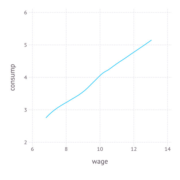
plot_c

4. Numerical simulation of optimal agent behavior under constraints

The replication code for this section is available here.

We now use constrained numerical optimization to generate optimal consumption and leisure data without analytically solving for the demand function. We begin by importing the data and the necessary packages:

####### Prepare for Numerical Optimization #########

using DataFrames
using JuMP
using Ipopt
df = readtable("consump_leisure.csv")
N = size(df)[1]

Using the JuMP syntax for non-linear modeling, first we define an empty model associated with the Ipopt solver, and then add $N$ values of $c_i$ and $N$ values of $l_i$ to the model:

m = Model(solver=IpoptSolver())    # define empty model solved by Ipopt algorithm
@defVar(m, c[i=1:N] >= 0)       # define positive consumption for each agent
@defVar(m, 0 <= l[i=1:N] <= 1)  # define leisure in [0,1] for each agent

This syntax is especially convenient, as it allows us to define vectors of parameters, each satisfying the natural inequality constraints. Next, we define the budget constraint, which also follows this convenient syntax:

 @addConstraint(m, c[i=1:N] .== (1.0-t)*(1.0-l[i]).*w[i] + e[i] )        # each agent must satisfy the budget constraint

Finally, we define a scalar-valued objective function, which is the sum of each individual’s utility:

 @setNLObjective(m, Max, sum{ g*log(c[i]) + (1-g)*log(l[i]) , i=1:N } )  # maximize the sum of utility across all agents

Notice that we can optimize one objective function instead of optimizing $N$ objective functions because the individual constrained maximization problems are independent across individuals, so the maximum of the sum is the sum of the maxima. Finally, we can apply the solver to this model and extract optimal consumption and leisure as follows:

 status = solve(m)                                                       # run numerical optimization c_opt = getValue(c)                                                     # extract demand for c l_opt = getValue(l)                                                     # extract demand for l

To make sure it worked, we compare the consumption extracted from this numerical approach to the consumption we generated previously using the true demand functions:

cor(c_opt,array(df[:consump]))
0.9999999998435865

Thus, we consumption values produced by the numerically optimizer’s approximation to the demand for consumption are almost identical to those produced by the true demand for consumption. Putting it all together, we create a function that can solve for optimal consumption and leisure given any particular values of $\gamma$ , $\tau$ , and $\epsilon$ :

 function hh_constrained_opt(g,t,w,e)      m = Model(solver=IpoptSolver())                                         # define empty model solved by Ipopt algorithm
  @defVar(m, c[i=1:N] >= 0)                                               # define positive consumption for each agent
  @defVar(m, 0 <= l[i=1:N] <= 1)                                          # define leisure in [0,1] for each agent
  @addConstraint(m, c[i=1:N] .== (1.0-t)*(1.0-l[i]).*w[i] + e[i] )        # each agent must satisfy the budget constraint
  @setNLObjective(m, Max, sum{ g*log(c[i]) + (1-g)*log(l[i]) , i=1:N } )  # maximize the sum of utility across all agents
  status = solve(m)                                                       # run numerical optimization
  c_opt = getValue(c)                                                     # extract demand for c
  l_opt = getValue(l)                                                     # extract demand for l
  demand = DataFrame(c_opt=c_opt,l_opt=l_opt)                             # return demand as DataFrame
end

hh_constrained_opt(gamma,tau,array(df[:wage]),array(df[:epsilon]))          # verify that it works at the true values of gamma, tau, and epsilon

5. Parallelized estimation by the Method of Simulated Moments

The replication codes for this section are available here.

We saw in the previous section that, for a given set of model parameters $\gamma$ and $\tau$ and a given draw of $\epsilon_{i}$ for each $i$ , we have enough information to simulation $c_{i}$ and $l_{i}$ , for each $i$ . Denote these simulated values by $\hat{c}_{i}\left(\epsilon;\gamma,\tau\right)$ and $\hat{l}_{i}\left(\epsilon;\gamma,\tau\right)$ . With these, we can define the moments,

$\hat{m}\left(\gamma,\tau\right)=\mathbb{E}_{\epsilon}\left[\begin{array}{c} \frac{1}{N}\sum_{i}\left[\hat{c}_{i}\left(\epsilon\right)-c_{i}\right]\\ \frac{1}{N}\sum_{i}\left[\hat{l}_{i}\left(\epsilon\right)-l_{i}\right] \end{array}\right]$

which is equal to zero under the model assumptions. A method of simulated moments (MSM) approach to estimate $\gamma$ and $\tau$ is then,

$\left(\hat{\gamma},\hat{\tau}\right)=\arg\min_{\gamma\in\left[0,1\right],\tau\in\left[0,1\right]}\hat{m}\left(\gamma,\tau\right)'W\hat{m}\left(\gamma,\tau\right)$

where $W$ is a $2\times2$ weighting matrix, which is only relevant when the number of moments is greater than the number of parameters, which is not true in our case, so $W$ can be ignored and the method of simulated moments simplifies to,

$\left(\hat{\gamma},\hat{\tau}\right)=\arg\min_{\gamma\in\left[0,1\right],\tau\in\left[0,1\right]}\left\{ \mathbb{E}_{\epsilon}\left[\frac{1}{N}\sum_{i}\left[\hat{c}_{i}\left(\epsilon\right)-c_{i}\right]\right]\right\} ^{2}+\left\{ \mathbb{E}_{\epsilon}\left[\frac{1}{N}\sum_{i}\left[\hat{l}_{i}\left(\epsilon\right)-l_{i}\right]\right]\right\} ^{2}$

Assuming we know the distribution of $\epsilon_i$ , we can simply draw many values of $\epsilon_i$ for each $i$ , and average the moments together across all of the draws of $\epsilon_i$ . This is Monte Carlo numerical integration. In Julia, we can create this objective function with a random draw of $\epsilon$ as follows:

function sim_moments(params)
  this_epsilon = randn(N)                                                     # draw random epsilon
  ggamma,ttau = params                                                        # extract gamma and tau from vector
  this_demand = hh_constrained_opt(ggamma,ttau,array(df[:wage]),this_epsilon) # obtain demand for c and l
  c_moment = mean( this_demand[:c_opt] ) - mean( df[:consump] )               # compute empirical moment for c
  l_moment = mean( this_demand[:l_opt] ) - mean( df[:leisure] )               # compute empirical moment for l
  [c_moment,l_moment]                                                         # return vector of moments
end

In order to estimate $\hat{m}\left(\gamma,\tau\right)$ , we need to run sim_moments(params) many times and take the unweighted average across them to achieve the expectation across $\epsilon_i$ . Because each calculation is computer-intensive, it makes sense to compute the contribution of $\hat{m}\left(\gamma,\tau\right)$ for each draw of $\epsilon_i$ on a different processor and then average across them.

Previously, I presented a convenient approach for parallelization in Julia. The idea is to initialize processors with the addprocs() function in an “outer” script, then import all of the needed data and functions to all of the different processors with the require() function applied to an “inner” script, where the needed data and functions are already managed by the inner script. This is incredibly easy and much simpler than the manual spawn-and-fetch approaches suggested by Julia’s official documentation.

In order to implement the parallelized method of simulated moments, the function hh_constrained_opt() and sim_moments() are stored in a file called est_msm_inner.jl. The following code defines the parallelized MSM and then minimizes the MSM objective using the optimize command set to use the Nelder-Mead algorithm from the Optim package:

####### Prepare for Parallelization #########

addprocs(3)                   # Adds 3 processors in parallel (the first is added by default)
print(nprocs())               # Now there are 4 active processors
require("est_msm_inner.jl")   # This distributes functions and data to all active processors

####### Define Sum of Squared Residuals in Parallel #########

function parallel_moments(params)
  params = exp(params)./(1.0+exp(params))   # rescale parameters to be in [0,1]
  results = @parallel (hcat) for i=1:numReps
    sim_moments(params)
  end
  avg_c_moment = mean(results[1,:])
  avg_l_moment = mean(results[2,:])
  SSR = avg_c_moment^2 + avg_l_moment^2
end

####### Minimize Sum of Squared Residuals in Parallel #########

using Optim
function MSM()
  out = optimize(parallel_moments,[0.,0.],method=:nelder_mead,ftol=1e-8)
  println(out)                                       # verify convergence
  exp(out.minimum)./(1.0+exp(out.minimum))           # return results in rescaled units
end

Parallelization is performed by the @parallel macro, and the results are horizontally concatenated from the various processors by the hcat command. The key tuning parameter here is numReps, which is the number of draws of $\epsilon$ to use in the Monte Carlo numerical integration. Because this example is so simple, a small number of repetitions is sufficient, while a larger number would be needed if $\epsilon$ entered the model in a more complicated manner. The process is run as follows and requires 268 seconds to run on my Macbook Air:

numReps = 12                                         # set number of times to simulate epsilon
gamma_MSM, tau_MSM = MSM()                           # Perform MSM
gamma_MSM
0.49994494921381816
tau_MSM
0.19992279518894465

Finally, given the MSM estimates of $\gamma$ and $\tau$ , we define the numerical derivative, $\frac{df(x)}{dx} \approx \frac{f(x+h)-f(x-h)}{2h}$ , for some small $h$ , as follows:

function Dconsump_Dtau(g,t,h)
  opt_plus_h = hh_constrained_opt(g,t+h,array(df[:wage]),array(df[:epsilon]))
  opt_minus_h = hh_constrained_opt(g,t-h,array(df[:wage]),array(df[:epsilon]))
  (mean(opt_plus_h[:c_opt]) - mean(opt_minus_h[:c_opt]))/(2*h)
end

barpsi_MSM = Dconsump_Dtau(gamma_MSM,tau_MSM,.1)
-5.016610457903023

Thus, we estimate the policy parameter $\bar\psi$ to be approximately $-5.017$ on average, while the true value is $\bar\psi = -\gamma \bar{w} = -(1/2)\times 10=-5$ , so the econometrician’s problem is successfully solved.

Bradley Setzler

Static and Ahead of Time (AOT) compiled Julia

On running Julia code without a JIT

Julia Computing carried out this work under contract from the Johns
Hopkins University Applied Physics Laboratory (JHU APL) for the Federal Aviation
Administration (FAA) to support its Traffic-Alert and Collision Avoidance
System (TCAS) program. JuliaCon 2015 had a very interesting talk by Robert Moss on this topic. Part of this work was also sponsored by Blackrock, Inc.

I’m often asked when I tell someone about Julia: “What makes it fast?” and “Why can’t <insert favorite dynamic language> do the same?” That’s not an easy question, since the answer has many parts, many of them nuanced and sometimes specific to a particular application – or even developer. Being fast is one benefit, but exploring the answer to this question also reveals some other applications: static compilation (i.e. removing the JIT dependency entirely), theorem proving, static memory allocation, and more! Answering this question requires an understanding of the traditional definitions of static vs. dynamic languages, and how Julia fits into that spectrum.

Many languages, including Julia, support templated code, macros, or other forms of source code generation. In traditional static languages, these have often been written in their own language dialect. This makes the distinction between the application and the generator functions immediately clear to the reader. But it also means the user must actually learn two dialects – and how they interact – to be fully proficient in the one language. This templating language may be simple (such as C Preprocessor macros), but may also be a full turing-complete interpreter (such as C++ templates).

Dynamic languages, by contrast, have commonly exposed similar functionality by providing an eval function. The reasoning is that since all code is being dynamically interpreted, there is no disadvantage for some of this code not being available to the compiler until “just-in-time” for the code to be executed. The distinction between application and generator is still fairly clear: the generator function ends with a call to eval.

It’s easy to blur the line between these two camps, however. For example, if a C++ program links against libclang (for example, the cling project), it is possible to program in the dynamic style. Or if a program written in a dynamic language doesn’t use eval, then it can be transpiled to avoid the runtime interpreter[1]. Julia embraces this hybridization. But to discuss the possibility of static compilation requires an understanding of this distinction between these two phases in the life cycle of the execution of code.

Julia follows in the Lisp tradition and provides tools for manipulating the language using the language itself. This can make it non-obvious to the reader which parts of the code are generators for application logic, and which parts of the program are the actual application logic. But this is also what complicates attempts to answer the initial question of whether Julia programs can be statically compiled – and what that question really means. If compilation is defined as finding the most efficient mapping of the source code onto the primitive instructions understood by the machine, then accurate static analysis is a prerequisite for the compiler to be able to optimize this translation. If the entire program can be statically transformed, then it is possible to generate compiled binaries and remove the runtime dependency for a parser / interpreter / compiler. And while compiler instruction selection is probably the most common static analysis, it is far from the only possible static analysis pass. For example, theorem proving, automated testing, and race detection are all active research areas.

A user’s first encounter with the Julia language is usually at the interactive REPL prompt, and then by writing script files in a similar style. At this top-level scope, all forms of dynamic evaluation are permitted: new types can be defined; functions created; variables can be modified and introspected via reflection; and modules can be defined and imported. However, once the user defines a local scope (for example, a function definition, let block, for loop), only static constructs can be used, with three exceptions provided for user flexibility: eval, macros, and generated functions. This is important, because it means that if the programmer avoids using these three dynamic constructs for the application logic, it is possible to statically analyze and compile the program generated as a result of running the user’s code file.

Let’s take a closer look at each of these cases:

A call to eval can be used as an escape hatch to invoke top-level expressions and the compiler from inside a function. This is akin to its purpose in a typical dynamic language (with the exception that it cannot introspect or modify a local variable, which many other languages do allow). Julia provides many constructs intended to help the user avoid needing this functionality, including closure (nested) functions, dynamic dispatch, type parameters, and macros.
Macro calls are demarcated by @ to distinguish them from regular function calls. They are functionally equivalent to the code templating features of many traditional static languages (albeit more ergonomic since they are implemented in Julia itself, in the style of Lisp). They are run after parsing, but before the code is executed. Indeed, there is no mechanism for invoking them at runtime so the existence of their definitions in a program does not cause problems.

Aside: If you’ve ever encountered the error: “unsupported or misplaced expression $”, this is specifically the runtime-macro behavior that is “unsupported”. Indeed, the syntax for a runtime invocation of a macro would be:
```
$(quote @macrocall $(args...) end)
```
Generated (aka staged) functions cannot be statically compiled. These functions are equivalent to calling eval on a new anonymous function computed as a function of the input types (a JIT-parsed lambda, if you will), and optionally memoizing the result. Therefore, it is possible to statically compile the memoization cache. This makes them, in this regard, superior to an unadorned eval call. But in the general case, generated functions are black boxes to the compiler and thus cannot be analyzed statically.

So there you have it. If you avoid eval and generated functions, any language – including Julia – can be statically compiled.

But that still leaves all of the important questions unanswered, such as: (a) why does this matter? (b) how can we use it? (c) what makes Julia special?

Julia is special because it was designed from the start as a dynamic language of the ilk described above, but one in which the programmer often can describe to the compiler the extent to which those features are used by a particular function. The built-in library of functionality (aka Base) was developed to provide this information and take advantage of these principles, which continues to influence authors of extension modules (aka packages) to also follow these principles. For example, the Julia community seems to have coined the term “type-stability” to describe a concept that static / compiled languages have historically enforced and dynamic / scripting languages have historically disregarded. These considerations are what allows Julia to claim both flexibility and speed. These concerns can be very difficult to retrofit onto a legacy codebase. Put another way, the speed potential of a language consists almost entirely of the properties that the compiler is able to prove ahead-of-time so that they don’t need to checked at runtime. And the flexibility comes from being able to get those runtime checks automatically whenever they are needed. Type-checking (and unboxing) is one aspect of these checks, but there are many other properties that can be computed such as stack allocation, statically-determined memory lifetimes, constant propagation, and call de-virtualization. (For a more complete discussion of these properties, see Oscar Blumberg’s Green Fairy Analysis)

This also means turning Julia code into Julia binaries requires no tricks, complicated incantations, or obscure limitations. In fact, the Julia runtime / compiler is already silently doing this for you on a regular basis. Sorry, if you were hoping for something really spectacular here – but that’s also not quite the end of the story, since we can exercise some direct control over it.

So now let’s pull back the covers on some of the options for the Julia binary. You may have glossed over this long list at some point (abridged):

~$ julia --help

julia [switches] -- [programfile] [args...]

-v, --version         	Display version information

-h, --help            	Print this message

-J, --sysimage <file> 	Start up with the given system image file

--precompiled={yes|no}	Use precompiled code from system image if available

--compilecache={yes|no}   Enable/disable incremental precompilation of modules

--startup-file={yes|no}   Load ~/.juliarc.jl

-e, --eval <expr>     	Evaluate <expr>

-E, --print <expr>    	Evaluate and show <expr>

-P, --post-boot <expr>	Evaluate <expr>, but don't disable interactive mode (deprecated, use -i -e instead)

-L, --load <file>     	Load <file> immediately on all processors

--compile={yes|no|all}	Enable or disable compiler, or request exhaustive compilation

--output-o name       	Generate an object file (including system image data)

--output-ji name      	Generate a system image data file (.ji)

--output-bc name      	Generate LLVM bitcode (.bc)

--output-incremental=no   Generate an incremental output file (rather than complete)

What you may not have been as readily aware of is that many of these options are used internally to handle various modes of operation. For instance, -p n (or addprocs(n)) will launch extra copies of julia on the indicated hosts with --worker.

The --output, --compile, and --sysimage are the ones that will be of primary interest for investigating the static compilations abilities of Julia.

When building the Julia language runtime from the .jl source files in base, the Julia runtime library code is run with a flag that tells it where to save the resulting application – code and variable declarations – after executing the input commands. The first call to ./julia during the source compilation evaluates the coreimg.jl file and writes a bytecode representation of the resulting Julia Inference analysis code to inference.ji:

./julia --output-ji inference.ji coreimg.jl

Then the system builds upon that image, to compile the entire Base system, by evaluating sysimg.jl in the runtime environment previously defined and saved to the inference.ji file:

./julia --output-o sys.o --sysimage inference.ji --startup-file=no 
	sysimg.jl

And since it compiled some of those functions to native code (due to directives in the precompile.jl file or other heuristics), that native code can be linked into a dynamic library for fast startup:

cc -shared -o sys.so sys.o -ljulia

In normal usage, the Julia runtime only invokes the compiler when a function is called. This is an intentional trade-off that incurs higher memory usage and longer compile times (aka JIT warm-up), with the expectation that the additional information from the presence of the types will enable the compiler to generate simpler code with fewer runtime operations – resulting in a net time savings. There’s another assumption in this behavior also: which is that the compiler will be available at runtime.

There are cases, however, where the user may want to or need to avoid running the compiler at runtime. The --compile=<yes|no|all> flag makes this possible (the default is yes). When Julia is run with the --compile=all flag, the compiler is invoked for all functions in the system image, so that the resulting sys-all.so binary contains native code for all functions defined in Base:

./julia --output-o sys-all.o --sysimage sys.so --startup-file=no 
	--compile=all --eval nothing
cc -shared -o sys-all.so sys-all.o -ljulia

This dynamic library no longer requires the compiler, which can be demonstrated by disabling the compiler by command line argument:

./julia --compile=no --sysimage sys-all.so

Or the compiler can be removed from the library entirely:

make JULIACODEGEN=none

resulting in a much smaller libjulia.so file –

– but which will throw an error if the system needs to use any methods at runtime that haven’t been pre-compiled to binary code:

I think it is worth mentioning here that the ./julia binary itself is actually just a very small utility wrapper for parsing the command line arguments and loading the actual Julia runtime from the sys.so dynamic library. This allows the same binary file to be used as both a dynamic library file and an executable, instead of needing to create two different output files. But the linker could instead be invoked slightly differently to embed the compiled code directly into the executable[2]:

cc -o julia-app sys.o repl.c -ljulia

Package code is handled similarly to the system image, so these same principles apply also to modules loaded with Base.__precompiled__(true) / Base.compilecache("Package"). These commands invoke the ./julia program in compiler-mode like the examples above, plus the addition of an incremental flag. This extra flag tells it that the output file should only include the delta of the code and definitions that are part of that package:

./julia --output-ji pkg.ji --sysimage sys.so --output-incremental=yes 
	pkg.jl

I think that about covers the current capabilities of Julia’s static compilation engine. Over time, I’m sure that I, and the rest of the team at Julia Computing Inc., will be adding many more under-the-hood features and optimizations to expand further on these powerful capabilities. This will allow Julia to be used on a broad variety of resource-constrained compute devices, many of which disallow JIT compilation or simply aren’t powerful enough for it to be beneficial – web-browsers (e.g. emscripten), smartphones, IoT devices (e.g. the Raspberry Pi), etc.

One other application of static analysis that I hadn’t yet touched on is the ability to convert Julia code to another language, such as C. In my next post, I plan to dive further into this capability and show how that can be done.

Supplemental Tools

Since Julia users often come to be aware of, and sometimes even fluent in, the esoterica of such tools as code_llvm and code_native, I feel it would be remiss of me if I didn’t point out that there are several standalone tools for analyzing the static files generated above. For complete documentation, refer to the llvm webpage for these tools.

To use most of these tools, you will need to start by re-running the command of interest above, and specifying --output-bc instead of (or in addition to) --output-o
llvm-dis : converts the .bc (llvm bitcode) binary file to .ll (llvm assembly text)
- roughly equivalent to code_llvm
llc : compiles a .bc or .ll file to .o (equivalent to the file from --output-o)
llvm-objdump : disassembles a .o file to .S
- roughly equivalent to code_native

[1]: This observation forms the basis of the JIT compilers for many popular languages such as Javascript.

[2]: There is near infinite variety in the flags that can be passed to cc to compile and link files. I’ve neglected to mention paths and a few flags that are frequently essential such as -L, -I, and -Wl,-rpath,$(pwd). I’m assuming here that the reader already has a toolchain configured for their purpose, so I’ve opted for trying to show a simple example clearly rather than trying to teach all of the nuances, which could fill a whole blog post of its own.

Introducing the Eclipse Julia plugin – JuliaDT

JuliaDT is an alpha release of an Eclipse-based IDE for Julia. Current trends in Big Data and Data Science make Julia a natural choice when tackling the latest business challenges. The plugin aims to make Julia’s strengths more readily accessible to an expanding community of developers.

The implementation is based on Eclipse DLTK. The design focuses on making Julia available in an enterprise setting, whilst ensuring that Julia-specific features remain handy and intuitive to use.

The IDE is work in progress. The roadmap includes extending existing features including outline and navigation as well as REPL, Plotting and Debugger support. The environment is downloadable as a plugin.

Feature	Screenshots
Interpreter Integration Reference a Julia installation and use it to execute programs directly within the environment. Also, to view associated console output.
Project and File Wizards Create Julia-specific Projects and Files
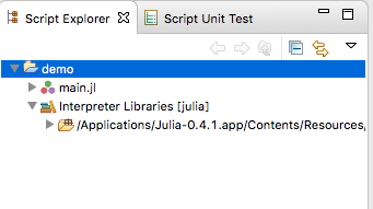
Project Explorer View project structure and navigate through associated files
Syntax Highlighting View program structure based on lexical analysis and keywords
Template Support Use shortcuts to view and quickly use appropriate Julia constructs
Auto-Completion Ensure syntactically correct endings
Outline View project types and functions
Open Type Browse/Navigate based on type name

We hope you find these features useful. All feedback is welcome. Updates on new features to follow in the coming months, so keep a look out. This work was carried out as part of a grant received from the Gordon and Betty Moore Foundation’s Data Driven Discovery Initiative.

juliabloggers.com

A Julia Language Blog Aggregator