Author Archives: Dean Markwick's Blog -- Julia

Converting an Edward Tutorial (Python) to Flux (Julia)

By: Dean Markwick's Blog -- Julia

Re-posted from: https://dm13450.github.io/2020/12/19/EdwardAndFlux.html

Here I’ll be showing you how to take a model built in Python with
Edward, convert it into Julia and perform the same type of inference
using Flux and Turing.jl.


Enjoy these types of posts? Then sign up for my newsletter.


Edward is a probabilistic programming language like Stan, PyMC3
and Turing.jl. You write a model and can perform statistical
inference on some data. Edward is a more ‘machine learning’ focused than Stan as
you can build neural nets and all the fun, modern techniques that the cool kids
are using. Flux.jl takes a similar ‘machine learning’ approach but this
time in Julia. Flux can build neural nets and also much
more. There is an intersection here between Edward and Flux, so it
makes sense to think that you can perform similar tasks. That is the whole point of this blog post, translating this
Edward tutorial: http://edwardlib.org/getting-started into Julia code
for Flux. So anyone reading this can get an idea of:

  • what Flux is all about,
  • how the Python Edward code can be transformed into Julia,
  • how to build a simple neural nets and infer the parameters in a Bayesian way.

I’ll start off by reproducing the model in Flux before calling on
Turing to do the Bayes bit. This is my first time writing about Flux,
so hopefully you’ll find this useful if it is also your first foray into doing some machine learning in Julia.

using Flux
using Plots
using Distributions

The original tutorial wants to learn the cos function of which we add some Gaussian noise.

f(x) = cos(x) + rand(Normal(0, 0.1))

xTrain = collect(-3:0.1:3)
yTrain = f.(xTrain)
plot(xTrain, yTrain, seriestype=:scatter, label="Train Data")
plot!(xTrain, cos.(xTrain), label="Truth")
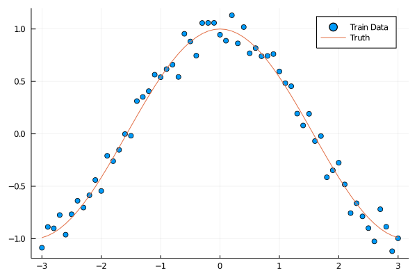
True data from the cos function

To build the neural net we chain two dense layers with tanh nonlinearities inbetween the layers. We use the mean square error as our loss function which we minimise using gradient descent. This is the most basic way in which you can build and train the neural net. Directly replicating what Edward does comes later, for now we just want to get things working.

With Flux you can specify what type of loss quite easily, with a list
of all that comes prepackaged found here
https://fluxml.ai/Flux.jl/stable/models/losses. But if none of those
take your fancy you can write your own and pass a simple Julia
function.

model = Chain(Dense(1, 2, tanh), Dense(2, 1))
loss(x, y) = Flux.Losses.mse(model(x), y)
optimiser = Descent(0.1);

Likewise for the optimiser. I’ve chose gradient descent, but again,
you can switch it out for a more advanced approach, such as ADAM. See
if any of those listed here
https://fluxml.ai/Flux.jl/stable/training/optimisers/ take your
fancy.

In short, the neural net takes one value as an input, passes through to two nodes on the hidden layer with a tanh activation function before outputting a single value as the output.

We now set up the training data. We take 100 random normal samples as our inputs, use our f function to generate the outputs and then repeat the dataset 100 times.

x = rand(Normal(), 100)
y = f.(x)
train_data = Iterators.repeated((Array(x'), Array(y')), 100);

We train the model for 10 epochs.

Flux.@epochs 10 Flux.train!(loss, Flux.params(model), train_data, optimiser)

Which takes no time at all to complete. We now want to make sure the
results are sensible and it has actually learnt the underlying
function.

yOut = zeros(length(xTrain))
for (i, x) in enumerate(xTrain)
    yOut[i] = model([xTrain[i]])[1]
end

plot(xTrain, yOut, label="Predicted")
plot!(xTrain, cos.(xTrain), label="True")
plot!(x, y, seriestype=:scatter, label="Data")
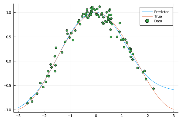
Predicted cruve from Flux

Everything looking good. Our neural net has found something similar to the true function, so hopefully you are convinced that we can now add a layer of complexity. Slight disagreement around the tails, but that is where we are lacking some data, so not too big of a deal.

Bayesian Neural Networks with Flux and Turing

All the above captured the spirit, but not the whole point of the
Edward tutorial, which is to create a Bayesian neural net. With a
Bayesian neural net there is a probability distribution over the
weights, rather than just singular values to maximise. In Julia, we
have to call upon our old friend Turing.jl. The Turing team have
written about Bayesian neural networks. I’ve taken some of that code and shuffled it about for this application.

using Turing

Firstly, have the parameters for each of the layers of the neural net. In total there are 6 parameters for the two layer model, so using the unpack function we take a vector of length 6 and break it up into the weights and biases for each layer which we then build in the nn_forward function.

function unpack(nn_params::AbstractVector)
    W₁ = reshape(nn_params[1:2], 2, 1);   
    b₁ = reshape(nn_params[3:4], 2)
    
    W₂ = reshape(nn_params[4:5], 1, 2); 
    b₂ = [nn_params[6]]
    
    return W₁, b₁, W₂, b₂
end

function nn_forward(xs, nn_params::AbstractVector)
    W₁, b₁, W₂, b₂ = unpack(nn_params)
    nn = Chain(Dense(W₁, b₁, tanh), Dense(W₂, b₂))
    return nn(xs)
end

These utility functions mean that we are tearing down the neural net and rebuilding it with the new parameters with each iteration. Turing deals with finding the best parameters by doing the Bayesian sampling (see my previous post on Hamilton MCMC sampling).

We think the 6 parameters of the neural net are drawn from a multivariate normal distribution and the parameters are all uncorrelated with each other. The observations are also from a normal distribution with mean from the neural net and variance \(\sigma\).

alpha = 0.1
sig = sqrt(1.0 / alpha)

@model bayes_nn(xs, ys) = begin
    
    nn_params ~ MvNormal(zeros(6), sig .* ones(6)) #Prior
    
    preds = nn_forward(xs, nn_params) #Build the net
    sigma ~ Gamma(0.01, 1/0.01) # Prior for the variance
    for i = 1:length(ys)
        ys[i] ~ Normal(preds[i], sigma)
    end
end;

Model built, we now want to use the NUTS algorithm to sample from the
posterior. Again, like Flux, you can use other sampling methods such as HMC
or Metropolis-Hastings.

N = 5000
ch1 = sample(bayes_nn(hcat(x...), y), NUTS(0.65), N);
ch2 = sample(bayes_nn(hcat(x...), y), NUTS(0.65), N);

We sample from posterior 5,000 times with two chains to check the convergence later. When selecting the final parameters we chose those that maximise the log posterior of the model. For each of the datapoints we add the prediction from the neural net.

lp, maxInd = findmax(ch1[:lp])

params, _ = ch1.name_map
bestParams = map(x-> ch1[x].data[maxInd], params[1:6])
plot(x, cos.(x), seriestype=:line, label="True")
plot!(x, Array(nn_forward(hcat(x...), bestParams)'), 
      seriestype=:scatter, label="MAP Estimate")
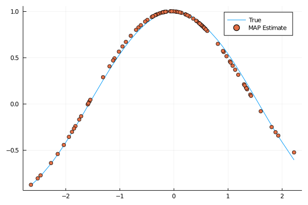
MAP estimate of the function

We can also sample from this posterior distribution by looking at the different parameters from the sampling process.

xPlot = sort(x)

sp = plot()

for i in max(1, (maxInd[1]-100)):min(N, (maxInd[1]+100))
    paramSample = map(x-> ch1[x].data[i], params)
    plot!(sp, xPlot, Array(nn_forward(hcat(xPlot...), paramSample)'), 
        label=:none, colour="blue")
    
end

plot!(sp, x, y, seriestype=:scatter, label="Training Data", colour="red")

sp
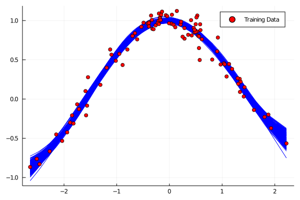
Posterior draws of the function

Again, looking sensible and representing the true underlying
function. Plus as we have done this using Bayes, we have a good
visualisation of the uncertainty of the model too.

And then finally we can assess how the chains of the model look and make a judgement on whether they have converged.

lPlot = plot(ch1[:lp], label="Chain 1", title="Log Posterior")
plot!(lPlot, ch2[:lp], label="Chain 2")

sigPlot = plot(ch1[:sigma], label= "Chain 1", title="Variance")
plot!(sigPlot, ch2[:sigma], label="Chain 2")

plot(lPlot, sigPlot)
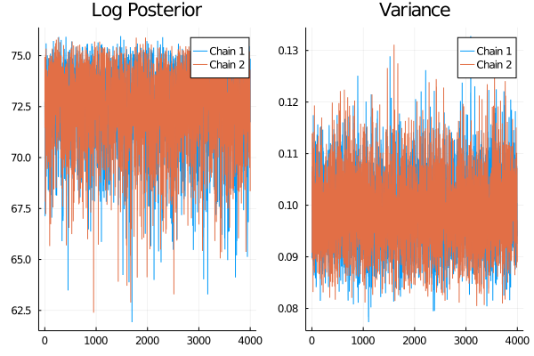
Chain convergence

Both chains are looking like they have converged, so we can trust our sampling process.

Conclusion

I actually surprised myself with how easy it was to build and sample
from the neural net in a Bayesian manner. I originally thought that I
would only be able to replicate the model using frequentist methods,
but not the Bayes steps. This just goes to show what a great job the Turing.jl team have done, making the whole model building and sampling simple.
So after reading this you can extended these models to bigger
and badder neural nets if that is what your problem needs. Easily swapping out
losses, optimisers and posterior sampling methods as needed.

This post also shows how easy it is to translate back and forth
between the different machine learning libraries and even programming
languages, although there is not too much of a difference between
Julia and Python. So if anyone out there is reading this trying to
decide on what language to pick up, I’d be biased and say Julia, but
really, you’ll be fine with either one.
Proper Bayesian Estimation of a Point Process in Julia

By: Dean Markwick's Blog -- Julia

Re-posted from: https://dm13450.github.io/2020/11/03/BayesPointProcess.html

I know how to use Stan and I know how to use Turing. But how do
those packages perform the posterior sampling for the underlying
models. Can I write a posterior distribution down and get
AdvancedHMC.jl to sample it? This is exactly what I want to do with
a point process where the posterior distribution of the model is a
touch more complicated than your typical regression problems.

This post will take you through my thought process and how you got from an idea, to a simulation of that idea, frequentist estimation of the simulated data and then a full Bayesian sampling of the problem.

But first, these are the Julia libraries that we will be using.

using Plots
using PlotThemes
using StatsPlots
using Distributions

Inhomogeneous Point Processes

A point process basically describes the time when something happens. That “thing” we can call an event and they happen between \(0\) and some maximum time \(T\). We describe the probability of an event happening at time \(t\) with an intensity \(\lambda\). Specifically we are going to use 4 different parameters for a polynomial.

\[\lambda (t) = \exp \left( \beta _0 + \beta _1 t + \beta _2 t^2 + \beta _3 ^2 t^3 \right)\]

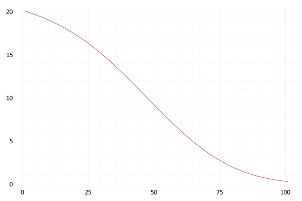
We take the exponent to ensure that the function is positive throughout the time period. What does this look like? We can simple plot the function from 0 to 100 with some random values for the \(\beta _i\)s.

λ(t::Number, params::Array{<:Number}) = exp(params[1] + params[2]*(t/100) + params[3]*(t/100)^2 + params[4]*(t/100)^3)
λ(t::Array{<:Number}, params::Array{<:Number}) = map(x-> λ(x, params), t)

testParams = [3, -0.5, -0.8, -2.9]
maxT = 100

plot(λ(collect(0:maxT), testParams), label=:none)

This looks like something that definitely changes over time. When
\(\lambda(t)\) is high we expect more events and likewise when it is
low there will be fewer events.

Simulating by Thinning

Let us simulate a point process using this intensity function. To do
so we use a procedure called thinning. This can be explained as a
three step process:

  1. Firstly simulate a constant Poisson process with intensity \(\lambda ^\star\) which is greater than \(\lambda (t)\) for all \(t\). This gives the un-thinned events, \(t^*_i\).
  2. For each un-thinned event calculate the probability it will become one of the final events as \(\frac{\lambda (t^*_i)}{\lambda ^\star}\).
  3. Sample from these probabilities to get the final events.

Simple enough to code up in a few lines of Julia.

lambdaMax = maximum(λ(collect(0:0.1:100), testParams)) * 1.1
rawEvents = rand(Poisson(lambdaMax * maxT), 1)[1]
unthinnedEvents = sort(rand(Uniform(0, maxT), rawEvents))
acceptProb = λ(unthinnedEvents, testParams) / lambdaMax
events = unthinnedEvents[rand(length(unthinnedEvents)) .< acceptProb];
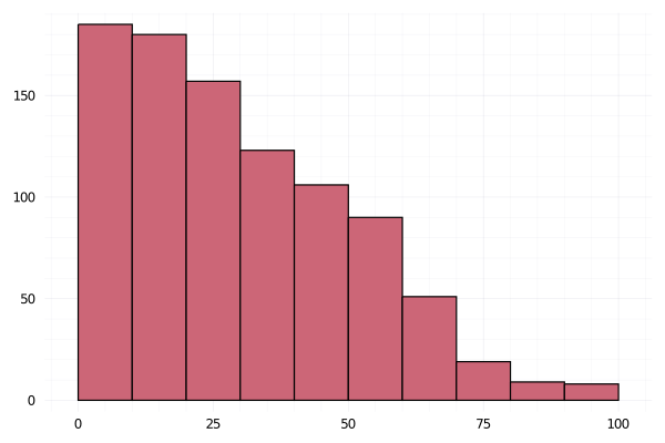
histogram(events,label=:none)

svg

A steady decreasing amount of events following the intensity function from above.

Maximum Likelihood Estimation

The log likelihood of a point process can be written as:

\[\mathcal{L} = \Sigma _{i = 1} ^N \log \lambda (t_i) – \int _0 ^T \lambda (t) \mathrm{d} t\]

Again, easy to write the code for this. The only technical difference is I am using the QuadGK.jl package to numerically integrate the function rather than doing the maths myself. This keeps it simple and also flexible if we decided to change the intensity function later.

function likelihood(params, rate, events, maxT)
    sum(log.(rate(events, params))) - quadgk(t-> rate(t, params), 0, maxT)[1]
end

For maximum likelihood estimation we simply pass this function through to an optimiser and find the maximum point. As optimize actually finds minimum points we have to invert the function.

using Optim
using QuadGK
opt = optimize(x-> -1*likelihood(x, λ, events, maxT), rand(4))
plot(λ(collect(0:maxT), testParams), label="True")
plot!(λ(collect(0:maxT), Optim.minimizer(opt)), label = "MLE")

svg

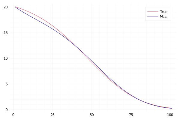
Not a bad result! Our estimated intensity function is pretty close to
the actual function. So now we know that we can both simulate from a inhomogeneous point
process and that our likelihood can infer the correct parameters.

Bayesian Inference

Now for the good stuff. All of the above is needed for the Bayesian inference procedure. If you can’t get the maximum likelihood working for a relatively simple problem like above, adding in the complications of Bayesian inference will just get you knotted up without any results. So with the good results from above let us proceed to the Bayes methods. With the AdvancedHMC.jl package I can use all the fancy MCMC algos and upgrade from the basic Metropolis Hastings sampling.

I’ve shamelessly copied the README from AdvancedHMC.jl and changed the bits needed for this problem.

using AdvancedHMC, ForwardDiff

D = 4; initial_params = rand(D)

n_samples, n_adapts = 5000, 2000

target(x) = likelihood(x, λ, events, maxT) + sum(logpdf.(Normal(0, 5), x))

metric = DiagEuclideanMetric(D)
hamiltonian = Hamiltonian(metric, target, ForwardDiff)

initial_ϵ = find_good_stepsize(hamiltonian, initial_params)
integrator = Leapfrog(initial_ϵ)
proposal = NUTS{MultinomialTS, GeneralisedNoUTurn}(integrator)
adaptor = StanHMCAdaptor(MassMatrixAdaptor(metric), StepSizeAdaptor(0.8, integrator))

samples1, stats1 = sample(hamiltonian, proposal, initial_params, 
                        n_samples, adaptor, n_adapts; progress=true);
samples2, stats2 = sample(hamiltonian, proposal, initial_params, 
                        n_samples, adaptor, n_adapts; progress=true);

Samples done, now to manipulate the results to get the parameter
estimation.

a11 = map(x -> x[1], samples1)
a12 = map(x -> x[1], samples2)
a21 = map(x -> x[2], samples1)
a22 = map(x -> x[2], samples2)
a31 = map(x -> x[3], samples1)
a32 = map(x -> x[3], samples2)
a41 = map(x -> x[4], samples1)
a42 = map(x -> x[4], samples2)

bayesEst = map( x -> mean(x[1000:end]), [a11, a21, a31, a41])
bayesLower = map( x -> quantile(x[1000:end], 0.25), [a11, a21, a31, a41])
bayesUpper = map( x -> quantile(x[1000:end], 0.75), [a11, a21, a31, a41])
density(a21, label="Chain 1")
density!(a22, label="Chain 2")
vline!([testParams[2]], label="True")
plot!(-4:4, pdf.(Normal(0, 5), -4:4), label="Prior")

svg

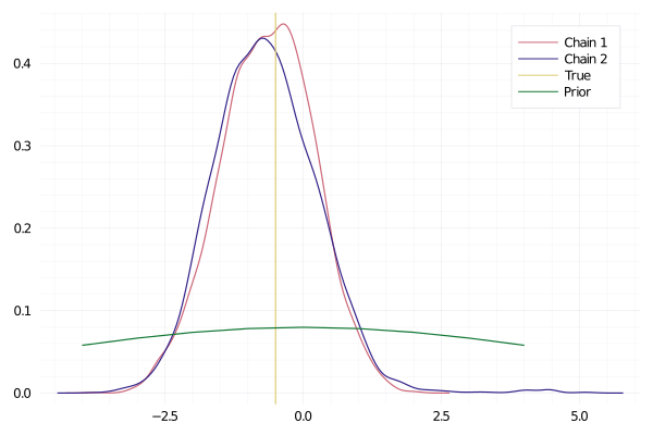
The chains have sampled correctly and are centered around the correct
value. Plus it’s suitably different from the prior, which shows it has
updated with the information from the events.

plot(a11, label="Chain 1")
plot!(a12, label="Chain 2")

svg

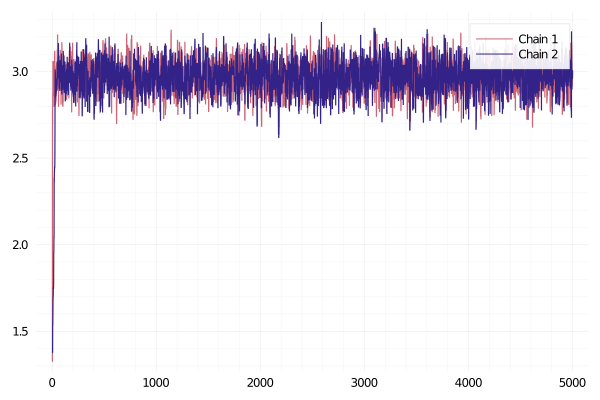
Looking at the convergence of the chains is also positive. So for this
simple model, everything looks like it has worked correctly.

plot(λ(collect(0:maxT), testParams), label="True")
plot!(λ(collect(0:maxT), Optim.minimizer(opt)), label = "MLE")
plot!(λ(collect(0:maxT), bayesEst), label = "Bayes")

svg

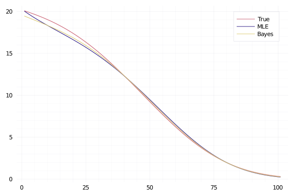
Again, the bayesian estimate of the function isn’t too far from the true intensity. Success!

Conclusion

So what have I learnt after writing all this:

  • AdvancedHMC.jl is easy to use and despite all the scary terms and settings you can get away with the defaults.

What I have hopefully taught you after reading this:

  • Point process simulation through thinning.
  • What the likelihood of a point process looks like.
  • Maximum likelihood using Optim.jl
  • How to use AdvancedHMC.jl for that point process likelihood to get the posterior distribution.

Hawkes Processes and DIC

By: Dean Markwick's Blog -- Julia

Re-posted from: https://dm13450.github.io/2020/08/26/Hawkes-and-DIC.html

My post on the deviance information criteria on my blog is one of the most popular ones I’ve ever written. So to take that theoretical concept and apply it to my new package HawkesProcesses.jl and show you how to construct the different functions needed to calculate the DIC.

Firstly, a recap on the DIC,

\[\begin{align*}
\text{DIC} & = – 2 \log p (y \mid \hat{\theta}) + 2 p_\text{DIC}, \\
p_\text{DIC} & = 2 \left( \log p(y \mid \hat{\theta} ) – \mathbb{E} \left[
\log p (y \mid \theta ) \right] \right),
\end{align*}\]

where these components are balancing up both the variation in the
parameters and how well the parameters fit the model to come up with a
number to assess the overall performance. Think of it as a more
intelligent likelihood calculation.

To calculate the DIC we need to construct the posterior distribution of the Hawkes process

\[p(\theta \mid y) = p(y \mid \theta) p(\theta),\]

where \(y\) are the event times. We’ve got the likelihood, \(p(y \mid \theta)\), already exposed from the package, so just have to add on the prior distribution of the parameters.

using HawkesProcesses
using Distributions

function posterior(events::Array{<:Number}, bg::Number, kappa::Number, kernelParam::Number, maxT::Number)
    kernel = Distributions.Exponential(1/kernelParam)
    lik::Float64 = HawkesProcesses.likelihood(events, bg, kappa, kernel, maxT)
    bgPrior = logpdf(Distributions.Gamma(0.01, 0.01), bg)
    kappaPrior = logpdf(Distributions.Gamma(0.01, 0.01), bg)
    kernPrior = logpdf(Distributions.Gamma(0.01, 0.01), kernelParam)
    lik + bgPrior + kappaPrior + kernPrior
end

This allows us evaluate the posterior for one sample, but what about multiple samples? Thankfully in Julia you don’t get punished for using for loops, so we can simply iterate through all the samples to calculate the posterior values.

function posterior(events::Array{<:Number}, bg::Array{<:Number}, kappa::Array{<:Number}, kernelParam::Array{<:Number}, maxT::Number)
    posteriorVals = Array{Float64}(undef, length(bg))
    for i in 1:length(bg)
        posteriorVals[i] = posterior(events, bg[i], kappa[i], kernelParam[i], maxT)
    end
    posteriorVals
end

We’ve got some functions, now just need some events and parameter samples to put everything into practise. Lets set up a standard Hawkes process.

bg = 0.5
kappa = 0.5
kernel = Distributions.Exponential(1/0.5)

simEvents = HawkesProcesses.simulate(bg, kappa, kernel, 1000)

bgSamples, kappaSamples, kernelSamples = HawkesProcesses.fit(simEvents, 1000, 1000)

bgSamples = bgSamples[500:end]
kappaSamples = kappaSamples[500:end]
kernelSamples = kernelSamples[500:end]

(mean(bgSamples), mean(kappaSamples), mean(kernelSamples))
(0.41608630082628845, 0.5735136278565907, 0.45633101066029247)

The final posterior samples are quite close the actually values, which is reassuring! We can now calculate the components of the DIC.

posteriorSamples = posterior(simEvents, bgSamples, kappaSamples, kernelSamples, 1000)
posteriorMean = posterior(simEvents, mean(bgSamples), mean(kappaSamples), mean(kernelSamples), 1000)
pdic = 2*(posteriorMean - mean(posteriorSamples))
dic = -2*mean(posteriorSamples) + 2*pdic
2147.693328671947

There we have it, simple to calculate and can now be used to critique the model. For example, we could fit another Hawkes model with a different kernel, calculate the DIC using the new samples and compare the values, the better fitting model will have a lower DIC value.

Bonus: Multithreading

using BenchmarkTools

The above function for calculating the posterior across the parameter samples can be easily parallelised in Julia 1.5 with some multithreading. Giving Julia access to the threads and the decorating the for loop with Threads.@threads will give us an easy speed boost in calculating the values.

To let Julia know you’ve got threads available you’ll need to prefix
your Julia startup:

> NUM_JULIA_THREADS=4 julia

To see if it worked then call (in Julia)

Threads.nthreads()

which should print out what ever number you set it too above (or the
maximum number of threads you’ve got on your machine).

We can now adapt the posterior function to take advantage of
threads.

function posterior_threaded(events::Array{<:Number}, bg::Array{<:Number}, kappa::Array{<:Number}, kernelParam::Array{<:Number}, maxT::Number)
    posteriorVals = Array{Float64}(undef, length(bg))
    Threads.@threads for i in 1:length(bg)
        posteriorVals[i] = posterior(events, bg[i], kappa[i], kernelParam[i], maxT)
    end
    posteriorVals
end

Call both functions to make sure they are compiled then we are ready to benchmark them using the same data that we calculated the DIC with.

posterior(simEvents, bgSamples, kappaSamples, kernelSamples, 1000)
posterior_threaded(simEvents, bgSamples, kappaSamples, kernelSamples, 1000);

And now to benchmark:

benchmarkBasic = @benchmarkable posterior($simEvents, $bgSamples, $kappaSamples, $kernelSamples, $1000)
benchmarkThreaded = @benchmarkable posterior_threaded($simEvents, $bgSamples, $kappaSamples, $kernelSamples, $1000)

benchmarkBasic = run(benchmarkBasic, seconds=300)
benchmarkThreaded = run(benchmarkThreaded, seconds=300)
judge(median(benchmarkThreaded), median(benchmarkBasic))
BenchmarkTools.TrialJudgement: 
  time:   -36.63% => improvement (5.00% tolerance)
  memory: +0.00% => minvariant (1.00% tolerance)

There we have it, using 4 threads instead of just the 1 gives us a 35% time improvement without too much hard work, which is nice.