Re-posted from: http://www.stochasticlifestyle.com/neural-jump-sdes-jump-diffusions-and-neural-pdes/
This is just an exploration of some new neural models I decided to jot down for safe keeping. DiffEqFlux.jl gives you the differentiable programming tools to allow you to use any DifferentialEquations.jl problem type (DEProblem) mixed with neural networks. We demonstrated this before, not just with neural ordinary differential equations, but also with things like neural stochastic differential equations and neural delay differential equations.
At the time we made DiffEqFlux, we were the “first to the gate” for many of these differential equations types and left it as an open question for people to find a use for these tools. And judging by the Arxiv papers that went out days after NeurIPS submissions were due, it looks like people now have justified some machine learning use cases for them. There were two separate papers on neural stochastic differential equations, showing them to be the limit of deep latent Gaussian models. Thus when you stick these new mathematical results on our existing adaptive high order GPU-accelerated neural SDE solvers, you get some very interesting and fast ways to learn some of the most cutting edge machine learning methods.
So I wanted to help you guys out with staying one step ahead of the trend by going to the next differential equations. One of the interesting NeurIPS-timed Arxiv papers was on jump ODEs. Following the DiffEqFlux.jl spirit, you can just follow the DifferentialEquations.jl tutorials on these problems, implement them, add a neural network, and it will differentiate through them. So let’s take it one step further and show an example of how you’d do that. I wanted to take a look at jump diffusions, or jump stochastic differential equations, which are exactly what they sound like. They are a mixture of these two methods. After that, I wanted to show how using some methods for stiff differential equations plus a method of lines discretization gives a way to train neural partial differential equations.
Instead of being fully defined by neural networks, I will also be showcasing how you can selectively make parts of a differential equation neuralitized and other parts pre-defined, something we’ve been calling mixed neural differential equations, so we’ll demonstrate a mixed neural jump stochastic differential equation and a mixed neural partial differential equation with fancy GPU-accelerated adaptive etc. methods. I’ll then leave as homework how to train a mixed neural jump stochastic partial differential equation with the fanciest methods, which should be easy to see from this blog post (so yes, that will be the MIT 18.337 homework). This blog post will highlight that these equations are all already possible within our framework, and will also show the specific places we see that we need to accelerate to really put these types of models into production.
Neural Jump Stochastic Differential Equations (Jump Diffusions)
To get to jump diffusions, let’s start with a stochastic differential equation. A stochastic differential equation is defined via

which is essentially saying that there is a deterministic term  and a continuous randomness term
  driven by a Brownian motion. Theorems like Donsker’s theorem can be thought of as a generalization of the central limit theorem, saying that continuous stochastic processes of some large class can be reinterpreted as this kind of process (due to the Gaussian-ness of Brownian motion), so in some sense this is a very large encompassing class. If you haven’t seen the previous blog post which mentions how to define neural SDEs, please check that out now. Let’s start with a code that uses reverse-mode automatic differentiation through a GPU-accelerated high order adaptive SDE solver. The code looks like:
using Flux, DiffEqFlux, StochasticDiffEq, Plots, DiffEqMonteCarlo

u0 = Float32[2.; 0.] |> gpu
datasize = 30
tspan = (0.0f0,1.0f0)

function trueODEfunc(du,u,p,t)
    true_A = [-0.1 2.0; -2.0 -0.1] |> gpu
    du .= ((u.^3)'true_A)'
end
t = range(tspan[1],tspan[2],length=datasize)
mp = Float32[0.2,0.2] |> gpu
function true_noise_func(du,u,p,t)
    du .= mp.*u
end
prob = SDEProblem(trueODEfunc,true_noise_func,u0,tspan)

# Take a typical sample from the mean
monte_prob = MonteCarloProblem(prob)
monte_sol = solve(monte_prob,SOSRI(),num_monte = 100)
monte_sum = MonteCarloSummary(monte_sol)
sde_data = Array(timeseries_point_mean(monte_sol,t))

dudt = Chain(x -> x.^3,
             Dense(2,50,tanh),
             Dense(50,2)) |> gpu
ps = Flux.params(dudt)
n_sde = x->neural_dmsde(dudt,x,mp,tspan,SOSRI(),saveat=t,reltol=1e-1,abstol=1e-1)

pred = n_sde(u0) # Get the prediction using the correct initial condition

dudt_(u,p,t) = Flux.data(dudt(u))
g(u,p,t) = mp.*u
nprob = SDEProblem(dudt_,g,u0,(0.0f0,1.2f0),nothing)

monte_nprob = MonteCarloProblem(nprob)
monte_nsol = solve(monte_nprob,SOSRI(),num_monte = 100)
monte_nsum = MonteCarloSummary(monte_nsol)
#plot(monte_nsol,color=1,alpha=0.3)
p1 = plot(monte_nsum, title = "Neural SDE: Before Training")
scatter!(p1,t,sde_data',lw=3)

scatter(t,sde_data[1,:],label="data")
scatter!(t,Flux.data(pred[1,:]),label="prediction")

function predict_n_sde()
  n_sde(u0)
end
loss_n_sde1() = sum(abs2,sde_data .- predict_n_sde())
loss_n_sde10() = sum([sum(abs2,sde_data .- predict_n_sde()) for i in 1:10])
Flux.back!(loss_n_sde1())

data = Iterators.repeated((), 10)
opt = ADAM(0.025)
cb = function () #callback function to observe training
  sample = predict_n_sde()
  # loss against current data
  display(sum(abs2,sde_data .- sample))
  # plot current prediction against data
  cur_pred = Flux.data(sample)
  pl = scatter(t,sde_data[1,:],label="data")
  scatter!(pl,t,cur_pred[1,:],label="prediction")
  display(plot(pl))
end

# Display the SDE with the initial parameter values.
cb()

Flux.train!(loss_n_sde1 , ps, Iterators.repeated((), 100), opt, cb = cb)
Flux.train!(loss_n_sde10, ps, Iterators.repeated((), 100), opt, cb = cb)

dudt_(u,p,t) = Flux.data(dudt(u))
g(u,p,t) = mp.*u
nprob = SDEProblem(dudt_,g,u0,(0.0f0,1.2f0),nothing)

monte_nprob = MonteCarloProblem(nprob)
monte_nsol = solve(monte_nprob,SOSRI(),num_monte = 100)
monte_nsum = MonteCarloSummary(monte_nsol)
#plot(monte_nsol,color=1,alpha=0.3)
p2 = plot(monte_nsum, title = "Neural SDE: After Training", xlabel="Time")
scatter!(p2,t,sde_data',lw=3,label=["x" "y" "z" "y"])

plot(p1,p2,layout=(2,1))

savefig("neural_sde.pdf")
savefig("neural_sde.png")
This just uses the diffeq_rd layer function to tell Flux to use reverse-mode AD (using Tracker.jl, unless you check out a bunch of weird Zygote.jl branches: wait for Zygote) and then trains the neural network using a discrete adjoint. While the previously posted example uses forward-mode, we have found that this is much much faster on neural SDEs, so if you’re trying to train them, I would recommend using this code instead (and I’ll get the examples updated).
Now to this equation let’s add jumps. A jump diffusion is defined like:

where  are the jump terms. The jump terms differ from the Brownian terms because they are non-continuous: they are zero except at countably many time points where you “hit” the equation with an amount
  . The timing at which these occur is based on an internal rate
  of the jump
  .
.
Jump diffusions are important because, just as there is a justification for the universality of stochastic differential equations, there is a justification here as well. The Levy Decomposition says that essentially any Markov process can be decomposed into something of this form. They also form the basis for many financial models, because for example changing regimes into a recession isn’t gradual but rather sudden. Models like Merton’s model thus use these as an essential tool in quantitative finance. So let’s train a neural network on that!
What we have to do is define jump processes and append them onto an existing differential equation. The documentation shows how to use the different jump definitions along with their pros and cons, so for now we will use ContinuousRateJump. Let’s define a ContinuousRateJump which has a constant rate and a neural network that decides what the effect of the jump () will be. To do this, you’d simply put the neural network in there:
rate(u,p,t) = 2.0
affect!(integrator) = (integrator.u = dudt2(integrator.u))
jump = ConstantRateJump(rate,affect!)
where dudt2 is another neural network, and then wrap that into a jump problem:
prob = SDEProblem(dudt_,g,gpu(param(x)),tspan,nothing)
jump_prob = JumpProblem(prob,Direct(),jump,save_positions=(false,false))
And of course you can make this fancier: just replace that rate 2.0 with another neural network, make the g(u,p,t) term also have a neural network, etc.: explore this as you wish and go find some cool stuff. Let’s just stick with this as our example though, but please go ahead and make these changes and allow DiffEqFlux.jl to help you to explore your craziest mathematical idea!
Now when you solve this, the jumps also occur along with the stochastic differential equation. To show what that looks like, let’s define a jump diffusion and solve it 100 times, taking its mean as our training data:
using Flux, DiffEqFlux, StochasticDiffEq, Plots, DiffEqMonteCarlo,
    DiffEqJump

u0 = Float32[2.; 0.]
datasize = 30
tspan = (0.0f0,1.0f0)

function trueODEfunc(du,u,p,t)
  true_A = [-0.1 2.0; -2.0 -0.1]
  du .= ((u.^3)'true_A)'
end
t = range(tspan[1],tspan[2],length=datasize)
const mp = Float32[0.2,0.2]
function true_noise_func(du,u,p,t)
  du .= mp.*u
end

true_rate(u,p,t) = 2.0
true_affect!(integrator) = (integrator.u[1] = integrator.u[1]/2)
true_jump = ConstantRateJump(true_rate,true_affect!)
prob = SDEProblem(trueODEfunc,true_noise_func,u0,tspan)
jump_prob = JumpProblem(prob,Direct(),true_jump,save_positions=(false,false))

# Take a typical sample from the mean
monte_prob = MonteCarloProblem(jump_prob)
monte_sol = solve(monte_prob,SOSRI(),num_monte = 100,parallel_type=:none)
plot(monte_sol,title="Training Data")

monte_sum = MonteCarloSummary(monte_sol)
sde_data = Array(timeseries_point_mean(monte_sol,t))
From the plot you can see wild discontinuities mixed in with an equation with continuous randomness. Just lovely.
A full code for training a neural jump diffusion thus is:
using Flux, DiffEqFlux, StochasticDiffEq, Plots, DiffEqMonteCarlo,
    DiffEqJump

u0 = Float32[2.; 0.] |> gpu
datasize = 30
tspan = (0.0f0,1.0f0)

function trueODEfunc(du,u,p,t)
  true_A = [-0.1 2.0; -2.0 -0.1] |> gpu
  du .= ((u.^3)'true_A)'
end
t = range(tspan[1],tspan[2],length=datasize)
const mp = Float32[0.2,0.2] |> gpu
function true_noise_func(du,u,p,t)
  du .= mp.*u
end

true_rate(u,p,t) = 2.0
true_affect!(integrator) = (integrator.u[1] = integrator.u[1]/2)
true_jump = ConstantRateJump(true_rate,true_affect!)
prob = SDEProblem(trueODEfunc,true_noise_func,u0,tspan)
jump_prob = JumpProblem(prob,Direct(),true_jump,save_positions=(false,false))

# Take a typical sample from the mean
monte_prob = MonteCarloProblem(jump_prob)
monte_sol = solve(monte_prob,SOSRI(),num_monte = 100,parallel_type=:none)
monte_sum = MonteCarloSummary(monte_sol)
sde_data = Array(timeseries_point_mean(monte_sol,t))

dudt = Chain(x -> x.^3,
           Dense(2,50,tanh),
           Dense(50,2)) |> gpu
dudt2 = Chain(Dense(2,50,tanh),
            Dense(50,2)) |> gpu
ps = Flux.params(dudt,dudt2)

g(u,p,t) = mp.*u
n_sde = function (x)
    dudt_(u,p,t) = dudt(u)
    rate(u,p,t) = 2.0
    affect!(integrator) = (integrator.u = dudt2(integrator.u))
    jump = ConstantRateJump(rate,affect!)
    prob = SDEProblem(dudt_,g,param(x),tspan,nothing)
    jump_prob = JumpProblem(prob,Direct(),jump,save_positions=(false,false))
    solve(jump_prob, SOSRI(); saveat=t ,abstol = 0.1, reltol = 0.1) |> Tracker.collect
end

pred = n_sde(u0) # Get the prediction using the correct initial condition

dudt__(u,p,t) = Flux.data(dudt(u))
rate__(u,p,t) = 2.0
affect!__(integrator) = (integrator.u = Flux.data(dudt2(integrator.u)))
jump = ConstantRateJump(rate__,affect!__)
nprob = SDEProblem(dudt__,g,u0,(0.0f0,1.0f0),nothing)
njump_prob = JumpProblem(prob,Direct(),jump, save_positions = (false,false))

monte_nprob = MonteCarloProblem(njump_prob)
monte_nsol = solve(monte_nprob,SOSRI(),num_monte = 1000,parallel_type=:none, abstol = 0.1, reltol = 0.1)
monte_nsum = MonteCarloSummary(monte_nsol)

#plot(monte_nsol,color=1,alpha=0.3)
p1 = plot(monte_nsum, title = "Neural Jump Diffusion: Before Training")
scatter!(p1,t,sde_data',lw=3)

scatter(t,sde_data[1,:],label="data")
scatter!(t,Flux.data(pred[1,:]),label="prediction")

function predict_n_sde()
    n_sde(u0)
end

loss_n_sde1() = sum(abs2,sde_data .- predict_n_sde())
 function loss_n_sde100()
    loss = sum([sum(abs2,sde_data .- predict_n_sde()) for i in 1:100])
    @show loss
    loss
end
function loss_n_sde500()
    loss = sum([sum(abs2,sde_data .- predict_n_sde()) for i in 1:500])
    @show loss
    loss
end
Flux.back!(loss_n_sde1())

data = Iterators.repeated((), 10)
opt = ADAM(0.025)
cb = function () #callback function to observe training
    sample = predict_n_sde()
    # loss against current data
    display(sum(abs2,sde_data .- sample))
    # plot current prediction against data
    cur_pred = Flux.data(sample)
    pl = scatter(t,sde_data[1,:],label="data")
    scatter!(pl,t,cur_pred[1,:],label="prediction")
    display(plot(pl))
end

# Display the SDE with the initial parameter values.
cb()

Flux.train!(loss_n_sde1 , ps, Iterators.repeated((), 100), opt, cb = cb)
Notice how it’s almost exactly the same as the SDE code but with the definition of the jumps. You still get the same high order adaptive GPU-accelerated (choice of implicit, etc.) SDE solvers, but now to this more generalized class of problems. Using the GPU gives a good speedup in the neural network case, but slows it down quite a bit when generating the training data since it’s not very parallel. Finding out new ways to use GPUs is one thing I am interested in perusing here. Additionally, using a lower tolerance StackOverflows Tracker.jl, which is something we have fixed with Zygote.jl and will be coming to releases once Zygote.jl on the differential equation solvers is more robust. Lastly, the plotting with GPU-based arrays is wonky right now, we’ll need to make the interface a little bit nicer. However, this is a proof of concept that this stuff does indeed work, though it takes awhile to train it to a “decent” loss (way more than the number of repetitions showcased in here).
[Note: you need to add using CuArrays to enable the GPU support. I turned it off by default because I was training this on my dinky laptop :)]
Neural Partial Differential Equations
Now let’s do a neural partial differential equation (PDE). We can start by pulling code from this older blog post on solving systems of stochastic partial differential equations with GPUs. Here I’m going to strip the stochastic part off, simply because I want to train this on my laptop before the flight ends, so again I’ll leave it as an exercise to do the same jump diffusion treatment to this PDE. Let’s start by defining the method of lines discretization for our PDE. If you don’t know what that is, please go read that blog post on defining SPDEs. What happens is the discretization gives you a set of ODEs to solve, which looks like:
using OrdinaryDiffEq, RecursiveArrayTools, LinearAlgebra,
DiffEqOperators, Flux, CuArrays
# Define the constants for the PDE
const α₂ = 1.0f0
const α₃ = 1.0f0
const β₁ = 1.0f0
const β₂ = 1.0f0
const β₃ = 1.0f0
const r₁ = 1.0f0
const r₂ = 1.0f0
const D = 100.0f0
const γ₁ = 0.1f0
const γ₂ = 0.1f0
const γ₃ = 0.1f0
const N = 100
const X = reshape([i for i in 1:N for j in 1:N],N,N) |> gpu
const Y = reshape([j for i in 1:N for j in 1:N],N,N) |> gpu
const α₁ = 1.0f0.*(X.>=80)
const Mx = Array(Tridiagonal([1.0f0 for i in 1:N-1],[-2.0f0 for i in 1:N],[1.0f0 for i in 1:N-1])) |> gpu
const My = copy(Mx)
Mx[2,1] = 2.0
Mx[end-1,end] = 2.0
My[1,2] = 2.0
My[end,end-1] = 2.0
# Define the initial condition as normal arrays
u0 = rand(Float32,N,N,3) |> gpu
const MyA = zeros(Float32,N,N) |> gpu
const AMx = zeros(Float32,N,N) |> gpu
const DA = zeros(Float32,N,N) |> gpu
# Define the discretized PDE as an ODE function
function f(_du,_u,p,t)
u = reshape(_u,N,N,3)
du= reshape(_du,N,N,3)
A = @view u[:,:,1]
B = @view u[:,:,2]
C = @view u[:,:,3]
dA = @view du[:,:,1]
dB = @view du[:,:,2]
dC = @view du[:,:,3]
mul!(MyA,My,A)
mul!(AMx,A,Mx)
@. DA = D*(MyA + AMx)
@. dA = DA + α₁ - β₁*A - r₁*A*B + r₂*C
@. dB = α₂ - β₂*B - r₁*A*B + r₂*C
@. dC = α₃ - β₃*C + r₁*A*B - r₂*C
end
# Solve the ODE
prob = ODEProblem(f,vec(u0),(0.0f0,100.0f0))
@time sol = solve(prob,BS3(), progress=true,saveat = 5.0)
@time sol = solve(prob,ROCK2(),progress=true,saveat = 5.0)
using Plots; pyplot()
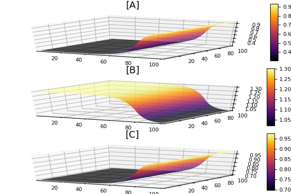
p1 = surface(X,Y,reshape(sol[end],N,N,3)[:,:,1],title = "[A]")
p2 = surface(X,Y,reshape(sol[end],N,N,3)[:,:,2],title = "[B]")
p3 = surface(X,Y,reshape(sol[end],N,N,3)[:,:,3],title = "[C]")
plot(p1,p2,p3,layout=grid(3,1))
savefig("neural_pde_training_data.png")
using DiffEqFlux, Flux
u0 = param(u0)
tspan = (0.0f0,100.0f0)
ann = Chain(Dense(3,50,tanh), Dense(50,3)) |> gpu
p1 = DiffEqFlux.destructure(ann)
ps = Flux.params(ann)
_ann = (u,p) -> reshape(p[3*50+51 : 2*3*50+50],3,50)*
tanh.(reshape(p[1:3*50],50,3)*u + p[3*50+1:3*50+50]) + p[2*3*50+51:end]
function dudt_(_u,p,t)
u = reshape(_u,N,N,3)
A = u[:,:,1]
DA = D .* (A*Mx + My*A)
_du = mapslices(x -> _ann(x,p),u,dims=3) |> gpu
du = reshape(_du,N,N,3)
x = vec(cat(du[:,:,1]+DA,du[:,:,2],du[:,:,3],dims=3))
end
prob = ODEProblem(dudt_,vec(Flux.data(u0)),tspan,Flux.data(p1))
@time diffeq_fd(p1,Array,length(u0)*length(0.0f0:5.0f0:100.0f0),prob,ROCK2(),progress=true,
saveat=0.0f0:5.0f0:100.0f0)
function predict_fd()
diffeq_fd(p1,Array,length(u0)*length(0.0f0:5.0f0:100.0f0),prob,ROCK2(),progress=true,
saveat=0.0f0:5.0f0:100.0f0)
end
function loss_fd()
_sol = predict_fd()
loss = sum(abs2,Array(sol) .- _sol)
@show loss
loss
end
loss_fd()
data = Iterators.repeated((), 10)
opt = ADAM(0.025)
Flux.train!(loss_fd, ps, data, opt)
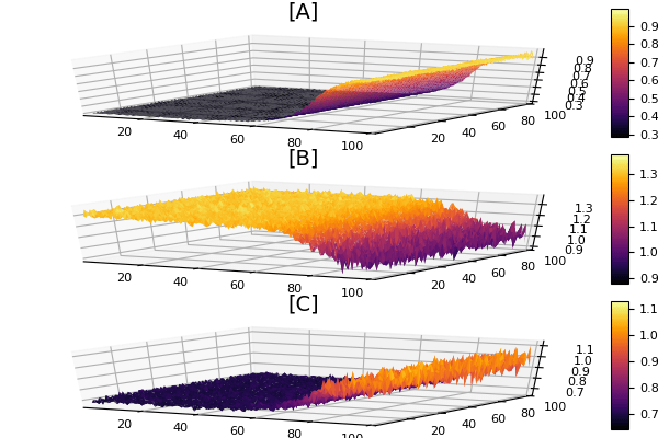
The interesting part of this neural differential equation is the local/global aspect of parts. The mapslices call makes it so that way there’s a local nonlinear function of 3 variables applied at each point in space. While it keeps the neural network small, this currently does not do well with reverse-mode automatic differentiation or GPUs. That isn’t a major problem here because, since the neural network is kept small in this architecture, the number of parameters is also quite small. That said, reverse-mode AD will be required for fast adjoint passes, so this is still a work in progress / proof of concept, with a very specific point made (all that’s necessary here is overloads to make mapslices work well).
One point that really came out of this was the ODE solver methods. The ROCK2 method is much faster when generating the training data and when running diffeq_fd. It was a difference of 3 minutes with ROCK2 vs 40 minutes with BS3 (on the CPU), showing how specialized methods really are the difference between the problem being solvable or not. The standard implicit methods like Rodas5 aren’t performing well here either since the 30,000×30,000 dense matrix, and I didn’t take the time to specify sparsity patterns or whatnot to actually make them viable competitors. So for the lazy neural ODE use with sparsity, ROCK2 seems like a very interesting option. This is a testament to our newest GSoC crew’s results since it’s one of the newer methods implemented by our student Deepesh Thakur. There are still a few improvements that need to be made to make the eigenvalue estimates more GPU-friendly as well, making this performance result soon carry over to GPUs as well (currently, the indexing in this part of the code gives it trouble, so a PR is coming probably in a week or so). Lastly, I’m not sure what’s a good picture for these kinds of things, so I’m going to have to think about how to represent a global neural PDE fit.
Conclusion
Have fun with this. There are still some rough edges, for example plotting is still a little wonky because all of the automatic DiffEq solution plotting seems to index, so the GPU-based arrays don’t like that (I’ll update that soon now that it’s becoming a standard part of the workflow). Use it as starter code and find some cool stuff. Note that the examples shown here are not the only ones that are possible. This all just uses Julia’s generic programming and differentiable programming infrastructure in order to automatically generate code that is compatible with GPUs and automatic differentiation, so it’s impossible for me to enumerate all of the possible combinations. That means there’s plenty of things to explore. These are very early preliminary results, but shows that these equations are all possible. These examples show some places where we want to continue accelerating by both improving the methods and their implementation details. I look forward to doing an update with Zygote soon.
CITATION:
Christopher Rackauckas, Neural Jump SDEs (Jump Diffusions) and Neural PDEs, The Winnower6:e155975.53637 (2019). DOI:10.15200/winn.155975.53637
This post is open to read and review on The Winnower.
The post Neural Jump SDEs (Jump Diffusions) and Neural PDEs appeared first on Stochastic Lifestyle.


![x \in [0,100]](https://i2.wp.com/www.stochasticlifestyle.com/wp-content/plugins/latex/cache/tex_944e326e3dddc5dae1278b292b330d64.gif)
![y \in [0,100]](https://i1.wp.com/www.stochasticlifestyle.com/wp-content/plugins/latex/cache/tex_43a28f59556b8f63f126a3ebe74b69ae.gif)


![[1,-2,1]](https://i0.wp.com/www.stochasticlifestyle.com/wp-content/plugins/latex/cache/tex_524fb89308e20bfe4e3ce99ffee459a6.gif)


![t \in [0,100]](https://i1.wp.com/www.stochasticlifestyle.com/wp-content/plugins/latex/cache/tex_e30a2ff606c68b20c3adbcdc6c97f8a3.gif)