Tag Archives: Julia

Use Julia to write code that runs on any GPU

By: Bart Schilperoort

Re-posted from: https://blog.esciencecenter.nl/use-julia-to-write-code-that-runs-on-any-gpu-3710cc8362da?source=rss----ab3660314556--julia

How to write Julia code than can run on any GPU, and why you would want to do that.

As the name implies, the main use of Graphics Processing Units is to process and render things to your screen, such as images, videos, or video games. Almost any device that has a display will have a GPU, although this can also come in the form of a chip integrated in the CPU instead of a separate graphics card. When using applications such as Google Maps, YouTube, or Netflix, the GPU renders the image/video to the screen more quickly and efficiently compared to the CPU. This can result in lower power consumption and a better user experience.
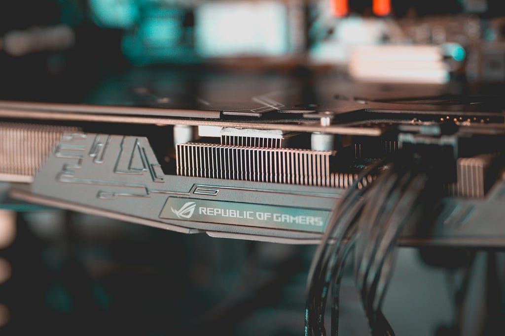
Photo by Dimitris Chapsoulas on Unsplash

To be able to render things to screen quickly, GPUs are able to do a lot of computations in parallel. Besides just graphics rendering, doing many computations in parallel can also come in use elsewhere, such as in (scientific) numerical models, and especially relevant recently, machine learning.

Before the release of Nvidia’s CUDA platform in 2007, people would use routines designed for graphics processing (like shaders), for non-graphics purposes such as numerical solvers for the Navier-Stokes equations. However, with CUDA, and soon after also OpenCL, it became more straightforward to write General Purpose GPU code.

When writing code for CUDA, you are locked into Nvidia designed GPUs, and the code cannot run elsewhere. With OpenCL, it was possible to write GPU code that can run on many platforms. While it can still work well on most hardware, it is seeing less and less support from Apple and Nvidia, who prefer to push their own proprietary platforms (Metal and CUDA).

Writing generic GPU code has a few benefits however, as you are not tied to a certain vendor, and there is a larger possible user base and thus more use cases. For example; accelerating a scientific model with GPU impacts both for laptop and high performance computing users.

To continue writing GPU code that can run on any hardware you can make use of Julia’s GPU ecosystem. With the KernelAbstractions.jl package you can write a kernel (a function that runs on a GPU and executes in parallel) that will work on any of the supported backends. Currently supported are Nvidia’s CUDA, AMD’s ROCm, Apple Metal, and Intel oneAPI. Which means that nearly all modern GPUs are supported, ranging from small laptops to supercomputers.

Julia example

To get started, after installing Julia, you can initialize arrays on the GPU with the appropriate backend package. As an example, I will use oneAPI, but the code will look the same for the other backends. The following line is the only one that’s machine dependent:

import oneAPI.oneArray as GPUArray

Having imported this, we can define arrays on the GPU. In this case a 2D matrix containing single-precision floating point numbers:

A = GPUArray(ones(Float32, 1024, 1024))

Now we can write a kernel. This example comes from the KernelAbstractions documentation, and will simply multiply every element of the matrix by 2:

using KernelAbstractions

@kernel function mul2_kernel(A)
I = @index(Global)
A[I] = 2 * A[I]
end

We can apply the kernel to the matrix A :

backend = get_backend(A)
mul2_kernel(backend, 64)(A, ndrange=size(A))

And that’s it! — Note that 64 is the “workgroup size”, i.e., the number of the array elements assigned to one work group. Tuning this parameter can make the kernel run faster.

For simple kernels, there is also the package AcceleratedKernels.jl, which allows you to convert normal loops into GPU accelerated loops by just changing a single line:

import AcceleratedKernels as AK

function cpu_copy!(dst, src)
for i in eachindex(src)
dst[i] = src[i]
end
end

function gpu_copy!(dst, src)
AK.foreachindex(src) do i
dst[i] = src[i]
end
end

The gpu_copy function will run on GPU if dst and src are GPU arrays. Otherwise the function will run on CPU.

Example packages

There are already some great packages that use KernelAbstractions to run on both CPU and any GPU. One of these is WaterLily.jl, a Computational Fluid Dynamics solver. Because it uses KernelAbstractions, they were able to run simulations not only on Nvidia GPUs, but also on AMD GPUs available on the LUMI supercomputer (one of the fastest in Europe!).

Simple 2D flow around the Julia logo, simulated using WaterLily.jl (source: WaterLily.jl)

The animation above can be generated on a laptop using the CPU or integrated graphics, but can be easily adapted to a higher resolution or 3D simulation to be run on a supercomputer.

The Julia GPU showcase page has many more examples ranging from climate models to bioinformatics.

Conclusion

By using Julia’s generic GPU framework, you can:

  • run and debug code locally, on your laptop using your CPU or GPU
  • have a larger community of users who can run the code on their own devices
  • deploy the code on any supercomputer, e.g., both Snellius (Nvidia GPUs) and LUMI (AMD GPUs)

So next time you need code to be fast and portable, consider using Julia to write code that can run fast, anywhere.


Use Julia to write code that runs on any GPU was originally published in Netherlands eScience Center on Medium, where people are continuing the conversation by highlighting and responding to this story.

Why Julia’s GPU Accelerated ODE Solvers are 20x-100x Faster than Jax and PyTorch

By: Christopher Rackauckas

Re-posted from: https://www.stochasticlifestyle.com/why-julias-gpu-accelerated-ode-solvers-are-20x-100x-faster-than-jax-and-pytorch/

You may have seen the benchmark results and thought, “how the heck are the Julia ODE solvers on GPUs orders of magnitude faster than the GPU-accelerated Python libraries, that can’t be true?” In this talk I will go into detail about the architectural differences between the Julia approaches to generating GPU-accelerated solvers vs the standard ML library approach to GPU usage. By the end of the talk you’ll have a good enough understanding of models of GPU acceleration to understand why this performance difference exists, and the many applications that can take advantage of this performance improvement.

The post Why Julia’s GPU Accelerated ODE Solvers are 20x-100x Faster than Jax and PyTorch appeared first on Stochastic Lifestyle.

How to Integrate Julia Code Within a Python Program

By: Great Lakes Consulting

Re-posted from: https://blog.glcs.io/julia-python-juliacall

This post was written by Steven Whitaker.

Ever wish your Python code could run fasteron heavy calculations or simulations?With juliacall,you can call Julia straight from Pythonand instantly access blazing-fast performanceand powerful scientific libraries,all without rewriting your existing code.Supercharge your Python workflows today andelevate your data science and engineering projectsto new heights!

In this Julia for Devs post,learn step-by-step how to install andutilize juliacall,enabling you toboost critical code performanceeffortlessly,without rewriting your entire project.Unlock the powerful combination ofPythons vast ecosystemand Julias speed,making it easy to experiment,optimize,or gradually migrate key components.

Let’s dig in!

Installing juliacall

Installation is a breeze,all you need is

pip install juliacall

You can test your installationby running the following in Python:

from juliacall import Main as jl

The first time this runs,it will install the Julia packagesneeded for communicatingbetween Julia and Python.

Then you can try it out:

import numpy as npA = np.array(jl.rand(5, 3))x = np.array(jl.randn(3))y = A @ x

Great,Julia-Python interoperabilityworks for this small example!Now let’s seehow we can extend thisto a larger example.

Calling Custom Code

In practice,we might have written some custom code in Juliathat we want to integrateinto our Python workflow.Let’s walk through the processof this integration.

Julia Code

Typically,the Julia code will be organizedinto a package,including its own package environmentand dependencies.

We’ll work with an examplethat runs a simulationusing OrdinaryDiffEq.jl and StaticArrays.jl.The example packagehas the following directory structure:

JuliaExample Project.toml src     JuliaExample.jl

The Project.toml has the following content:

name = "JuliaExample"uuid = "0b6476de-1cea-499f-93be-749bc74a9c07"authors = ["Author Name <[email protected]>"]version = "0.1.0"[deps]OrdinaryDiffEq = "1dea7af3-3e70-54e6-95c3-0bf5283fa5ed"StaticArrays = "90137ffa-7385-5640-81b9-e52037218182"

And JuliaExample.jl contains:

module JuliaExampleusing OrdinaryDiffEq: ODEProblem, Tsit5, solveusing StaticArrays: SVectorstruct Params    ::Float64    ::Float64    ::Float64endfunction f(u, p, t)    (; , , ) = p    dx =  * (u[2] - u[1])    dy = u[1] ( - u[3]) - u[2]    dz = u[1] * u[2] -  * u[3]    return SVector(dx, dy, dz)endfunction simulate(u0, t_start, t_end, , , )    u0 = SVector{3, Float64}(u0)    tspan = (t_start, t_end)    p = Params(, , )    prob = ODEProblem{false}(f, u0, tspan, p)    sol = solve(prob, Tsit5())endend

Python Code

We have our custom Julia code,so now let’s seewhat our Python workflow looks likethat calls out to Julia.

We’ll have our code organizedin the following directory structure:

python_example pyproject.toml scripts    run.py src     python_example         __init__.py         analysis.py

The main functionality of our Python codeis in analysis.py:

from juliacall import Main as jljl.seval("using JuliaExample: simulate")import numpy as npimport matplotlib.pyplot as pltdef simulate(*args):    result = jl.simulate(*args)    t = np.array(result.t)    sol = np.array([np.array(u) for u in result.u])    return t, soldef plot_results(t, sol):    plt.figure(figsize=(10, 6))    labels = ["x", "y", "z"]    colors = ["tab:blue", "tab:orange", "tab:green"]    for i in range(3):        plt.plot(t, sol[:, i], label=labels[i], color=colors[i])    plt.xlabel("Time [s]")    plt.ylabel("Value")    plt.title("Solution Components Over Time")    plt.legend()    plt.grid(True)    plt.tight_layout()    plt.show()

This code provides two functions:one for calling out to Juliato run a simulation,and another for plotting the simulation results.

Let’s break down some of this codeto see how Julia is incorporated:

  • from juliacall import Main as jl
    We saw this earlier;this is how to load juliacall.
  • jl.seval("using JuliaExample: simulate")
    Here,we load our Julia package,specifically bringing the function simulateinto scope.
  • The Python function simulatecalls the Julia simulate,passing along all its inputs:
    result = jl.simulate(*args)
    The Python functionthen does some processingto convert the Julia resultsinto something more easily utilizedby further Python processing.

This functionality is exercisedin the run.py script:

from python_example import simulate, plot_resultsimport numpy as npu0 = np.array([1, 0, 0])t_start = 0t_end = 100alpha = 10beta = 28gamma = 8/3t, sol = simulate(u0, t_start, t_end, alpha, beta, gamma)plot_results(t, sol)

Finally,for completeness,here’s __init__.py:

from .analysis import simulate, plot_results

Finding Julia

We have all our code set up,so now we need Pythonto be able to find the Julia codeso we can call out to it.In other words,we need the Julia package environmentused by juliacallto have JuliaExample as a dependency.

We can accomplish thisby creating a juliapkg.json filein our Python project directory(i.e., python_example/juliapkg.json).The file should contain the following JSON:

{    "packages": {        "JuliaExample": {            "uuid": "0b6476de-1cea-499f-93be-749bc74a9c07",            "path": "path/to/JuliaExample",            "dev": true        }    }}

Note that the uuid hereneeds to match the uuidin JuliaExample/Project.toml.And the "path" and "dev": true fields are necessarybecause our Julia package exists locally on our machine;it is not a registered Julia package.See the juliacall docsfor more information about juliapkg.json.

Putting It Together

Now we have all the components we need:Python code to run,Julia code to call out to,and juliapkg.json to tell juliacallwhere to find our Julia code.

So, what happens when we run run.py?

The first time it is run,juliacall will set up the Julia package environment,installing the dependencies of JuliaExample.Then, the script proceeds to run the simulation(calling out to Julia to do so)and plot the results:

Simulation results

Awesome,we now have a working exampleshowing how to call out to Juliafrom a Python project!

Summary

In this post,we saw how to install and use juliacallto call out to Julia from within Python.We looked at a trivial exampleas well as a more realistic exampleof integrating custom Julia codeinto a Python project.

What custom Julia codedo you want to integrateinto your Python projects?Contact us, and we can make it happen!

Additional Links

  • PythonCall.jl
    • One cool thing about juliacallis it is maintained in the same GitHub repoas PythonCall,which is the recommended wayto call Python code from Julia.
  • GLCS Modeling & Simulation
    • Connect with us for Julia Modeling & Simulation consulting.
]]>