Tag Archives: Julia

Six of One (Plot), Half-Dozen of the Other

By: randyzwitch - Articles

Re-posted from: http://badhessian.org/2014/07/six-of-one-plot-half-dozen-of-the-other/

This is a guest post by Randy Zwitch (@randyzwitch), a digital analytics and predictive modeling consultant in the Greater Philadelphia area. Randy blogs regularly about Data Science and related technologies at http://randyzwitch.com. He’s blogged at Bad Hessian before here.

WordPress Stats - Visitors vs. Views
WordPress Stats – Visitors vs. Views

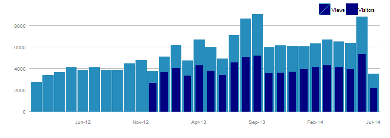
For those of you with WordPress blogs and have the Jetpack Stats module installed, you’re intimately familiar with this chart. There’s nothing particularly special about this chart, other than you usually don’t see bar charts with the bars shown superimposed.

I wanted to see what it would take to replicate this chart in R, Python and Julia. Here’s what I found. (download the data).

R: ggplot2

Although I prefer to use other languages these days for my analytics work, there’s a certain inertia/nostalgia that when I think of making charts, I think of using ggplot2 and R. Creating the above chart is pretty straightforward, though I didn’t quite replicate the chart, as I couldn’t figure out how to make my custom legend not do the diagonal bar thing.

The R Cookbook talks about a hack to remove the diagonal lines from legends, so I don’t feel too bad about not getting it. I also couldn’t figure out how to force ggplot2 to give me the horizontal line at 10000. If anyone in the R community knows how to fix these, let me know!
(Pythonistas: I’m aware of the ggplot port by Yhat; functionality I used in my R code is still in TODO, so I didn’t pursue plotting with ggplot in Python)

R: Base Graphics

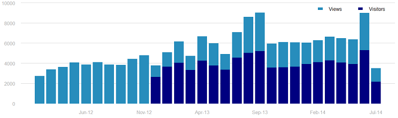
Of course, not everyone finds ggplot2 to be easy to understand, as it requires a different way of thinking about coding than most ‘base’ R functions. To that end, there are the base graphics built into R, which produced this plot: wordpress-base-rWhile I was able to nearly replicate the WordPress chart (except for the feature of having the dark bars slightly smaller width than the lighter), the base R syntax is horrid. The abbreviations for plotting arguments are indefensible, the center and width keywords seem to shift the range of the x-axis instead of changing the actual bar width, and in general, the experience plotting using base R was the worst of the six libraries I evaluated.
Python: matplotlib

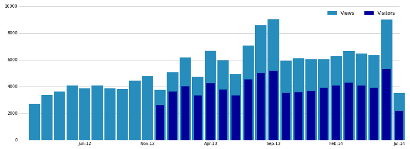
In the past year or so, there’s been quite a lot of activity towards improving the graphics capabilities in Python. Historically, there’s been a lot of teeth-gnashing about matplotlib being too low-level and hard to work with, but with enough effort, the results are quite pleasant. Unlike with ggplot2 and base R, I was able to replicate all the features of the WordPress plot:wordpress-matplotlib
Python: Seaborn

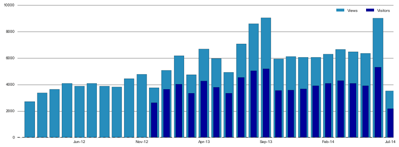
One of the aforementioned improvements to matplotlib is Seaborn, which promises to be a higher-level means of plotting data than matplotlib, as well as adding new plotting functionality common in statistics and research. Re-creating this plot using Seaborn is a waste of the additional functionality of Seaborn, and as such, I found it more difficult to make this plot using Seaborn than I did with matplotlib.

To replicate the plot, I ended up hacking a solution together using both Seaborn functionality and matplotlib in order to be able to set bar width and to create the legend, which defeats the purpose of using Seaborn in the first place.
Julia: Gadfly

In the Julia community, Gadfly is clearly the standard for plotting graphics. Supporting d3.js, PNG, PS, and PDF, Gadfly is built to work with many popular back-end environments. I was able to replicate everything about the WordPress graph except for the legend:wordpress-julia-gadflyWhile Gadfly took a line or two more than base R in terms of fewest lines of code, I find the Gadfly syntax significantly more pleasant to work with.

Julia: Plot.ly

Plot.ly is an interesting ‘competitor’ in this challenge, as it’s not a language-specific package per-se. Rather, Plot.ly is a means of specifying plots using JSON, with lightweight Julia/Python/MATLAB/R wrappers. I was able to replicate nearly everything about the WordPress plot, with the exception of not having a line at 10000, having the legend vertical instead of horizontal and I couldn’t figure out how to set the bar widths separately. wordpress-julia-plotly

And The Winner Is…matplotlib?!

If you told me at the beginning of this exercise that matplotlib (and by extension, Seaborn) would be the only library that I would be able to replicate all the features of the WordPress graph, I wouldn’t have believed it. And yet, here we are. ggplot2 was certainly very close, and I’m certain that someone knows how to fix the diagonal line issue. I suspect I could submit an issue ticket to Gadfly.jl to get the feature added to create custom legends (and for that matter, make the request of Plot.ly for horizontal legends), so in the future there could be feature parity using these two libraries as well.

I hope we all agree there’s no hope for Base Graphics in R besides quick throwaway plots.

In the end, the best thing I can say from this exercise is that the analytics community is fortunate to have so many talented people working to provide these amazing visualization libraries. This graph was rather pedestrian in nature, so I didn’t even scratch the surface of what these various libraries can do. Even beyond the six libraries I chose, there are others I didn’t choose, including: prettyplotlib (Python), Bokeh (Python), Vincent (Python), rCharts (R), ggvis (R), Winston (Julia), ASCII Plots (Julia) and probably even more that I’m not even aware of! All free and open-source and miles apart from terrible looking Microsoft graphics in Excel and Powerpoint.

Julia for Data Science

Julia is a great language for doing data science. With its C-like speed, familiar Matlab/Numpy style API, extensive standard library, metaprogramming and parallel processing capabilities, and growing set of machine learning libraries, it is rapidly gaining ground within the data science community. In this IJulia notebook we’ll go through brief introductions to the language and some of the packages available for data wrangling, visualization, analysis and prediction. Stay tuned for more to come.

Cobbling together parallel random number generation in Julia

I’m starting to work on some computationally demanding projects, (Monte Carlo simulations of bootstraps of out-of-sample forecast comparisons) so I thought I should look at Julia some more. Unfortunately, since Julia’s so young (it’s almost at version 0.3.0 as I write this) a lot of code still needs to be written. Like Random Number Generators (RNGs) that work in parallel. So this post describes an approach that parallelizes computation using a standard RNG; for convenience I’ve put the code (a single function) is in a grotesquely ambitiously named package on GitHub: ParallelRNGs.jl. (Also see this thread on the Julia Users mailing list.)

A few quick points about RNGs and simulations. Most econometrics papers have a section that examines the performance of a few estimators in a known environment (usually the estimators proposed by the paper and a few of the best preexisting estimators). We do this by simulating data on a computer, using that data to produce estimates, and then comparing those estimate to the parameters they’re estimating. Since we’ve generated the data ourselves, we actually know the true values of those parameters, so we can make a real comparison. Do that for 5000 simulated data sets and you can get a reasonably accurate view of how the statistics might perform in real life.

For many reasons, it’s useful to be able to reproduce the exact same simulations again in the future. (Two obvious reasons: it allows other researchers to be able to reproduce your results, and it can make debugging much faster when you discover errors.) So we almost always use pseudo Random Number Generators that use a deterministic algorithm to produce a stream of numbers that behaves in important ways like a stream of independent random values. You initialize these RNGs by setting a starting value (the “pseudo” aspect of the RNGs is implicit from now on) and anyone who has that starting value can reproduce the identical sequence of numbers that you generated. A popular RNG is the “Mersenne Twister,” and “popular” is probably an understatement: it’s the default RNG in R, Matlab, and Julia. And (from what I’ve read; this isn’t my field at all) it’s well regarded for producing a sequence of random numbers for statistical simulations.

But it’s not necessarily appropriate for producing several independent sequences of random numbers. Which is vitally important because I have an 8 core workstation that needs to run lots of simulations, and I’d like to execute 1/8th of the total simulations on each of its cores.

There’s a common misconception that you can get independent random sequences just by choosing different initial values for each sequence, but that’s not guaranteed to be true. There are algorithms for choosing different starting values that are guaranteed to produce independent streams for the Mersenne Twister (see this research by one of the MT’s inventors), but they aren’t implemented in Julia yet. (Or in R, as far as I can tell; they use a different RNG for parallel applications.) And it turns out that Mersenne Twister is the only RNG that’s included in Julia so far.

So, this would be a perfect opportunity for me to step up and implement some of these advanced algorithms for the Mersenne Twister. Or to implement some of the algorithms developed by L’Ecuyer and his coauthors, which are what R uses. And there’s already C code for both options.

But I haven’t done that yet. I’m lazy busy.

Instead, I’ve written an extremely small function that wraps Julia’s default RNG, calls it from the main process alone to generate random numbers, and then sends those random numbers to each of the other processes/cores where the rest of the simulation code runs. The function’s really simple:

function replicate(sim::Function, dgp::Function, n::Integer)
    function rvproducer()
        for i=1:n
            produce(dgp())
        end
    end
    return(pmap(sim, Task(rvproducer)))
end

That’s all. If you’re not used to Julia, you can ignore the “::Function” and the “::Integer” parts of the arguments. Those just identify the datatype of the argument and you can read it as “dgp_function” if you want (and explicitly providing the types like this is optional anyway). So, you give “replicate” two functions: “dgp” generates the random numbers and “sim” does the remaining calculations; “n” is the number of simulations to do. All of the work is done in “pmap” which parcels out the random numbers and sends them to different processors. (There’s a simplified version of the source code for pmap at that link.)

And that’s it. Each time a processor finishes one iteration, pmap calls dgp() again to generate more random numbers and passes them along. It automatically waits for dgp() to finish, so there are no race conditions and it produces the exact same sequence of random numbers every time. The code is shockingly concise. (It shocked me! I wrote it up assuming it would fail so I could understand pmap better and I was pretty surprised when it worked.)

A quick example might help clear up it’s usage. We’ll write a DGP for the bootstrap:

const n = 200     #% Number of observations for each simulation
const nboot = 299 #% Number of bootstrap replications
addprocs(7)       #% Start the other 7 cores
dgp() = (randn(n), rand(1:n, (n, nboot)))

The data are iid Normal, (the “randn(n)” component) and it’s an iid nonparametric bootstrap (the “rand(1:n, (n, nboot))”, which draws independent values from 1 to n and fills them into an n by nboot matrix). Oh, and there’s a good reason for those weird “#%” comments; “#” is Julia’s comment character, but WordPress doesn’t support syntax highlighting for Julia, so we’re pretending this is Matlab code. And “%” is Matlab’s comment character, which turns the comment green.

We’ll use a proxy for some complicated processing step:

@everywhere function sim(x)
    nboot = size(x[2], 2)
    bootvals = Array(Float64, nboot)
    for i=1:nboot
        bootvals[i] = mean(x[1][x[2][:,i]])
    end
    confint = quantile(bootvals, [0.05, 0.95])
    sleep(3) #% not usually recommended!
    return(confint[1] < 0 < confint[2])
end

So “sim” calculates the mean of each bootstrap sample and calculates the 5th and 95th percentile of those simulated means, giving a two-sided 90% confidence interval for the true mean. Then it checks whether the interval contains the true mean (0). And it also wastes 3 seconds sleeping, which is a proxy for more complicated calculations but usually shouldn’t be in your code. The initial “@everywhere” is a Julia macro that loads this function into each of the separate processes so that it’s available for parallelization. (This is probably as good a place as any to link to Julia’s “Parallel Computing” documentation.)

Running a short Monte Carlo is simple:

julia> srand(84537423); #% Initialize the default RNG!!!
julia> @time mc1 = mean(replicate(sim, dgp, 500))

elapsed time: 217.705639 seconds (508892580 bytes allocated, 0.13% gc time)
0.896 #% = 448/500

So, about 3.6 minutes and the confidence intervals have coverage almost exactly 90%.

It’s also useful to compare the execution time to a purely sequential approach. We can do that by using a simple for loop:

function dosequential(nsims)
    boots = Array(Float64, nsims)
    for i=1:nsims
        boots[i] = sim(dgp())
    end
    return boots
end

And, to time it:

julia> dosequential(1); #% Force compilation before timing
julia> srand(84537423); #% Reinitialize the default RNG!!!
julia> @time mc2 = mean(dosequential(500))

elapsed time: 1502.038961 seconds (877739616 bytes allocated, 0.03% gc time)
0.896 #% = 448/500

This takes a lot longer: over 25 minutes, 7 times longer than the parallel approach (exactly what we’d hope for, since the parallel approach runs the simulations on 7 cores). And it gives exactly the same results since we started the RNG at the same initial value.

So this approach to parallelization is great… sometimes.

This approach should work pretty well when there aren’t that many random numbers being passed to each processor, and when there aren’t that many simulations being run; i.e. when “sim” is an inherently complex calculation. Otherwise, the overhead of passing the random numbers to each process can start to matter a lot. In extreme cases, “dosequential” can be faster than “replicate” because the overhead of managing the simulations and passing around random variables dominates the other calculations. In those applications, a real parallel RNG becomes a lot more important.

If you want to play with this code yourself, I made a small package for the replicate function: ParallelRNGs.jl on GitHub. The name is misleadingly ambitious (ambitiously misleading?), but if I do add real parallel RNGs to Julia, I’ll put them there too. The code is still buggy, so use it at your own risk and let me know if you run into problems. (Filing an issue on GitHub is the best way to report bugs.)

P.S. I should mention again that Julia is an absolute joy of a language. Package development isn’t quite as nice as in Clojure, where it’s straightforward to load and unload variables from the package namespace (again, there’s lots of code that still needs to be written). But the actual language is just spectacular and I’d probably want to use it for simulations even if it were slow. Seriously: seven lines of new code to get an acceptable parallel RNG.

Filed under: Blog Tagged: econometrics, julia, programming