Tag Archives: Julia

Selection Bias Corrections in Julia, Part 1

Re-posted from: https://juliaeconomics.com/2014/09/02/selection-bias-corrections-in-julia-part-1/

Selection bias arises when a data sample is not a random draw from the population that it is intended to represent. This is especially problematic when the probability that a particular individual appears in the sample depends on variables that also affect the relationships we wish to study. Selection bias corrections based on models of economic behavior were pioneered by the economist James J. Heckman in his seminal 1979 paper.

For an example of selection bias, suppose we wish to study the effectiveness of a treatment (a new medicine for patients with a particular disease, a preschool curriculum for children facing particular disadvantages, etc.). A random sample is drawn from the population of interest, and the treatment is randomly assigned to a subset of this sample, with the remaining subset serving as the untreated (“control”) group. If the subsets followed instructions, then the resulting data would serve as a random draw from the data generating process that we wish to study.

However, suppose the treatment and control groups do not comply with their assignments. In particular, if only some of the treated benefit from treatment while the others are in fact harmed by treatment, then we might expect the harmed individuals to leave the study. If we accepted the resulting data as a random draw from the data generating process, it would appear that the treatment was much more successful than it actually was; an individual who benefits is more likely to be present in the data than one who does not benefit.

Conversely, if treatment were very beneficial, then some individuals in the control group may find a way to obtain treatment, possibly without our knowledge. The benefits received by the control group would make it appear that the treatment was less beneficial than it actually was; the receipt of treatment is no longer random.

In this tutorial, I present some parameterized examples of selection bias. Then, I present examples of parametric selection bias corrections, evaluating their effectiveness in recovering the data generating processes. Along the way, I demonstrate the use of the GLM package in Julia. A future tutorial demonstrates non-parametric selection bias corrections.

Example 1: Selection on a Normally-Distributed Unobservable

Suppose that we wish to study of the effect of the observable variable $X_{i}$ on $Y_i$ . The data generating process is given by,

$Y_i=\beta_0+X_i\beta_1+\epsilon_i$ ,

where $X_i$ and $\epsilon_i$ are independent in the population. Because of this independence condition, the ordinary least squares estimator would be unbiased if the data $(Y,X)$ were drawn randomly from the population. However, suppose that the probability that individual $i$ were in the data set $\mathcal{S}$ were a function of $X$ and $\epsilon$ . For example, suppose that,

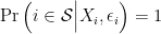
$\Pr\left( i \in \mathcal{S}\Big| X_i,\epsilon_i\right)=1$ if $X_i > \epsilon_i$ ,

and the probability is zero otherwise. This selection rule ensures that, among the individuals in the data (the $i$ in $\mathcal{S}$ ), the covariance between $X$ and $\epsilon$ will be positive, even though the covariance is zero in the population. When $X$ covaries positively with $\epsilon$ , then the OLS estimate of $\beta_1$ is biased upward, i.e., the OLS estimator converges to a value that is greater than $\beta_1$ .

To see the problem, consider the following simulation of the above process in which $X$ and $\epsilon$ are drawn as independent standard normal random variables:

srand(2)
N = 1000
X = randn(N)
epsilon = randn(N)
beta_0 = 0.
beta_1 = 1.
Y = beta_0 + beta_1.*X + epsilon
populationData = DataFrame(Y=Y,X=X,epsilon=epsilon)
selected = X.>epsilon
sampleData = DataFrame(Y=Y[selected],X=X[selected],epsilon=epsilon[selected])

There are 1,000 individuals in the population data, but 492 of them are selected to be included in the sample data. The covariance between X and epsilon in the population data is,

cov(populationData[:X],populationData[:epsilon])
0.00861456704877879

which is approximately zero, but in the sample data, it is,

cov(sampleData[:X],sampleData[:epsilon])
0.32121357192108513

which is approximately 0.32.

Now, we regress $Y$ on $X$ with the two data sets to obtain,

linreg(array(populationData[:X]),array(populationData[:Y]))
2-element Array{Float64,1}:
 -0.027204
  1.00882

linreg(array(sampleData[:X]),array(sampleData[:Y]))
2-element Array{Float64,1}:
 -0.858874
  1.4517

where, in Julia 0.3.0, the command array() replaces the old command matrix() in converting a DataFrame into a numerical Array. This simulation demonstrates severe selection bias associated with using the sample data to estimate the data generating process instead of the population data, as the true parameters, $\beta_0=0,\beta_1=1$ , are not recovered by the sample estimator.

Correction 1: Heckman (1979)

The key insight of Heckman (1979) is that the correlation between $X$ and $\epsilon$ can be represented as an omitted variable in the OLS moment condition,

$\mathbb{E}\left[Y_i\Big|X_i,i\in\mathcal{S}\right]=\mathbb{E}\left[\beta_0 + \beta_1X_i+\epsilon_i\Big|X_i,i\in\mathcal{S}\right]=\beta_0 + \beta_1X_i+\mathbb{E}\left[\epsilon_i\Big|X_i,i\in\mathcal{S}\right]$ ,

Furthermore, using the conditional density of the standard Normally distributed $\epsilon$ ,

$\mathbb{E}\left[\epsilon_i\Big|X_i,i\in\mathcal{S}\right]=\mathbb{E}\left[\epsilon_i\Big|X_i,X_i>\epsilon_i\right]=\frac{-\phi\left(X_i\right)}{\Phi\left(X_i\right)}$ .

which is called the inverse Mills ratio, where $\phi$ and $\Phi$ are the probability and cumulative density functions of the standard normal distribution. As a result, the moment condition that holds in the sample is,

$\mathbb{E}\left[Y_i\Big|X_i,i\in\mathcal{S}\right]=\beta_0 + \beta_1X_i+\frac{-\phi\left(X_i\right)}{\Phi\left(X_i\right)}$

Returning to our simulation, the inverse Mills ratio is added to the sample data as,

sampleData[:invMills] = -pdf(Normal(),sampleData[:X])./cdf(Normal(),sampleData[:X])

Then, we run the regression corresponding to the sample moment condition,

linreg(array(sampleData[[:X,:invMills]]),array(sampleData[:Y]))
3-element Array{Float64,1}:
 -0.166541
  1.05648
  0.827454

We see that the estimate for $\beta_1$ is now 1.056, which is close to the true value of 1, compared to the non-corrected estimate of 1.452 above. Similarly, the estimate for $\beta_0$ has improved from -0.859 to -0.167, when the true value is 0. To see that the Heckman (1979) correction is consistent, we can increase the sample size to $N=100,000$ , which yields the estimates,

linreg(array(sampleData[[:X,:invMills]]),array(sampleData[:Y]))
3-element Array{Float64,1}:
 -0.00417033
  1.00697
  0.991503

which are very close to the true parameter values.

Note that this analysis generalizes to the case in which $X$ contains $K$ variables and the selection rule is,

$\delta_0 + \delta_1 X_1 + \delta_2 X_2 + \ldots + \delta_K X_k > \epsilon$ ,

which is the case considered by Heckman (1979). The only difference is that the coefficients $\delta_k$ must first be estimated by regressing an indicator for $i \in \mathcal{S}$ on $X$ , then using the fitted equation within the inverse Mills ratio. This requires that we observe $X$ for $i \notin \mathcal{S}$ . Probit regression is covered in a slightly different context below.

As a matter of terminology, the process of estimating $\delta$ is called the “first stage”, and estimating $\beta$ conditional on the estimates of $\delta$ is called the “second stage”. When the coefficient on the inverse Mills ratio is positive, it is said that “positive selection” has occurred, with “negative selection” otherwise. Positive selection means that, without the correction, the estimate of $\beta_1$ would have been upward-biased, while negative selection results in a downward-biased estimate. Finally, because the selection rule is driven by an unobservable variables $\epsilon$ , this is a case of “selection on unobservables”. In the next section we consider a case of “selection on observables”.

Example 2: Probit Selection on Observables

Suppose that we wish to know the mean and variance of $Y$ in the population. However, our sample of $Y$ suffers from selection bias. In particular, there is some $X$ such that the probability of observing $Y$ depends on $X$ according to,

$\Pr\left(i\in\mathcal{S}\Big| X_i\right)=F\left(X_i\right)$ ,

where $F$ is some function with range $[0,1]$ . Notice that, if $Y$ and $X$ were independent, then the resulting sample distribution of $Y$ would be a random draw from the population (marginal distribution) of $Y$ . Instead, we suppose $\mathrm{Cov}\left(X,Y\right)\neq 0$ . For example,

srand(2)
N = 10000
populationData = DataFrame(rand(MvNormal([0,0.],[1 .5;.5 1]),N)')
names!(populationData,[:X,:Y])

mean(array(populationData),1)
1x2 Array{Float64,2}:
 -0.0281916  -0.022319

cov(array(populationData))
2x2 Array{Float64,2}:
 0.98665   0.500912
 0.500912  1.00195

In this simulated population, the estimated mean and variance of $Y$ are -0.022 and 1.002, and the covariance between $X$ and $Y$ is 0.501. Now, suppose the probability that $Y_i$ is observed is a probit regression of $X_i$ ,

$\Pr\left( i\in\mathcal{S}\Big| X_i \right) = \Phi\left( \beta_0 + \beta_1 X_i \right)$ ,

where $\Phi$ is the CDF of the standard normal distribution. Letting $D_i=1$ indicate that $i \in \mathcal{S}$ , we can generate the sample selection rule $D$ as,

beta_0 = 0
beta_1 = 1
index = (beta_0 + beta_1*data[:X])
probability = cdf(Normal(0,1),index)
D = zeros(N)
for i=1:N
    D[i] = rand(Bernoulli(probability[i]))
end
populationData[:D] = D
sampleData = populationData
sampleData[D.==0,:Y] = NA

The sample data has missing values in place of $Y_i$ if $D_i=0$ . The estimated mean and variance of $Y$ in the sample data are 0.275 (which is too large) and 0.862 (which is too small).

Correction 2: Inverse Probability Weighting

The reason for the biased estimates of the mean and variance of $Y$ in Example 2 is sample selection on the observable $X$ . In particular, certain values of $Y$ are over-represented due to their relationship with $X$ . Inverse probability weighting is a way to correct for the over-representation of certain types of individuals, where the “type” is captured by the probability of being included in the sample.

In the above simulation, conditional on appearing in the population, the probability that an individual of type $X_i=1$ is included in the sample is 0.841. By contrast, the probability that an individual of type $X_i=0$ is included in the sample is 0.5, so type $X_i$ is over-represented by a factor of 0.841/0.5 = 1.682. If we could reduce the impact that type $X_i=1$ has in the computation of the mean and variance of $Y$ by a factor of 1.682, we would alter the balance of types in the sample to match the balance of types in the population. Inverse probability weighting generalizes this logic by weighting each individual’s impact by the inverse of the probability that this individual appears in the sample.

Before we can make the correct, we must first estimate the probability of sample inclusion. This can be done by fitting the probit regression above by least-squares. For this, we use the GLM package in Julia, which can be installed the usual way with the command Pkg.add(“GLM”).

using GLM
Probit = glm(D ~ X, sampleData, Binomial(), ProbitLink())
DataFrameRegressionModel{GeneralizedLinearModel,Float64}:

Coefficients:
             Estimate Std.Error  z value Pr(>|z|)
(Intercept)  0.114665  0.148809 0.770554   0.4410
X             1.14826   0.21813  5.26414    1e-6

estProb = predict(Probit)
weights = 1./estProb[D.==1]/sum(1./estProb[D.==1])

which are the inverse probability weights needed to match the sample distribution to the population distribution.

Now, we use the inverse probability weights to correct the mean and variance estimates of $Y$ ,

correctedMean = sum(sampleData[D.==1,:Y].*weight)
-0.024566923132025013

correctedVariance = (N/(N-1))*sum((sampleData[D.==1,:Y]-correctedMean).^2.*weight)
1.0094029613131092

which are very close to the population values of -0.022319 and 1.00195. The logic here extends to the case of multivariate $X$ , as more coefficients are added to the Probit regression. The logic also extends to other functional forms of $F$ , for example, switching from Probit to Logit is achieved by replacing the ProbitLink() with LogitLink() in the glm() estimation above.

Example 3: Generalized Roy Model

For the final example of this tutorial, we consider a model which allows for rich, realistic economic behavior. In words, the Generalized Roy Model is the economic representation of a world in which each individual must choose between two options, where each option has its own benefits, and one of the options costs more than the other. In math notation, the first alternative, denoted $D_i=1$ , relates the outcomes $Y_i$ to the individual’s observable characteristics, $X_i$ , by,

$Y_{1,i} = \mu_1\left(X_i\right)+U_{1,i}$ .

Similarly, the second alternative, denoted $D_i=0$ , relates $Y_i$ to $X_i$ , by,

$Y_{0,i} = \mu_0\left(X_i\right)+U_{0,i}$ .

The value of $Y_i$ that appears in our sample is thus given by,

$Y_i = D_iY_{1,i} + (1-D_i)Y_{0,i}$ .

Finally, the value of $D_i$ is chosen by individual $i$ according to,

$D_i=1$ if $Y_{1,i}-Y_{0,i}-C_i>0$ ,

where $C_i$ is the cost of choosing the alternative $D_i=1$ and is given by,

$C_i = \mu_C\left(X_i,Z_i\right)+U_{C,i}$ ,

where $Z$ contains additional characteristics of $i$ that are not included in $X$ .

We assume that the data only contains $Y_i,D_i,X_i,Z_i$ ; it does not contain the variables $Y_{i,1},Y_{i,0},U_{i,1},U_{i,0},U_{i,C}$ or the functions $\mu_1,\mu_0,\mu_C$ . Assuming that the three $\mu$ functions follow the linear form and that the unobservables $U$ are independent and Normally distributed, we can simulate the data generating process as,

srand(2)
N = 1000
sampleData = DataFrame(rand(MvNormal([0,0.],[1 .5; .5 1]),N)')
names!(sampleData,[:X,:Z])
U1 = rand(Normal(0,.5),N)
U0 = rand(Normal(0,.7),N)
UC = rand(Normal(0,.9),N)
betas1 = [0,1]
betas0 = [.3,.2]
betasC = [.1,.1,.1]
Y1 = betas1[1] + betas1[2].*sampleData[:X] + U1
Y0 = betas0[1] + betas0[2].*sampleData[:X] + U0
C = betasC[1] + betasC[2].*sampleData[:X] + betasC[3].*sampleData[:Z] + UC
D = Y1-Y0-C.>0
Y = D.*Y1 + (1-D).*Y0
sampleData[:D] = D
sampleData[:Y] = Y

In this simulation, about 38% of individuals choose the alternative $D_i=1$ . About 10% of individuals choose $D_i=0$ even though they receive greater benefits under $D_i=1$ due to the high cost $C_i$ associated with $D_i=1$ .

Solution 3: Heckman Correction for Generalized Roy Model

The identification of this model is attributable to Heckman and Honore (1990). Estimation proceeds in steps. The first step is to notice that the left- and right-hand terms in the following moment equation motivate a Probit regression:

$\mathbb{E}\left[D_i\Big|X_i,Z_i\right]=\Pr\left(\mu_D\left(X_i,Z_i\right)>U_{D,i}\Big|X_i,Z_i\right)=\Phi\left(\mu_D\left(X_i,Z_i\right)\right)$ ,

where $U_{D,i}\equiv -\left(U_{1,i}-U_{0,i}-U_{C,i}\right)/\sigma_D\sim\mathcal{N}\left(0,1\right)$ is the negative of the total error term arising in the equation that determines $D_i$ above, $\sigma_D \equiv \sqrt{\mathrm{Var}\left(U_{1,i}-U_{0,i}-U_{C,i}\right)}$ , and,

$\mu_D\left(X,Z\right) \equiv \left([1,X]\beta_1 -[1,X]\beta_0 -[1,X,Z]\beta_C\right)/\sigma_D \equiv [1,X,Z]\beta_D$ ,

In the simulation above, $\beta_D = [-.4,.7,-.1]/\sqrt{.5+.7+.9}\approx[-0.276,0.483,-0.069]$ . We can estimate $\beta_D$ from the Probit regression of $D$ on $X$ and $Z$ .

betasD = coef(glm(D~X+Z,sampleData,Binomial(),ProbitLink()))
3-element Array{Float64,1}:
 -0.299096
  0.59392 
 -0.103155

Next, notice that,

$\mathbb{E}\left[Y_i\Big|D_i=1,X_i,Z_i\right] =[1,X_i]\beta_1+\mathbb{E}\left[U_{1,i}\Big|D_i=1,X_i,Z_i\right]$ ,

where,

$\mathbb{E}\left[U_{1,i}\Big|D_i=1,X_i,Z_i\right] =\mathbb{E}\left[U_{1,i}\Big|\mu_D\left(X_i,Z_i\right)>U_{i,D},X_i,Z_i\right]=\rho_1 \frac{-\phi\left(\mu_D\left(X_i,Z_i\right)\right)}{\Phi\left(\mu_D\left(X_i,Z_i\right)\right)}$ ,

which is the inverse Mills ratio again, where $\rho_1 \equiv \frac{\mathrm{Cov}\left(U_1,U_D\right)}{\mathrm{Var}\left(U_D\right)}$ . Substituting in the estimate for $\beta_D$ , we consistently estimate $\beta_1$ :

fittedVals = hcat(ones(N),array(sampleData[[:X,:Z]]))*betasD

sampleData[:invMills1] = -pdf(Normal(0,1),fittedVals)./cdf(Normal(0,1),fittedVals)

correctedBetas1 = linreg(array(sampleData[D,[:X,:invMills1]]),vec(array(sampleData[D,[:Y]])))
3-element Array{Float64,1}:
  0.0653299
  0.973568 
 -0.135445

To see how well the correction has performed, compare these estimates to the uncorrected estimates of $\beta_1$ ,

biasedBetas1 = linreg(array(sampleData[D,[:X]]),vec(array(sampleData[D,[:Y]])))
2-element Array{Float64,1}:
 0.202169
 0.927317

Similar logic allows us to estimate $\beta_0$ :

sampleData[:invMills0] = pdf(Normal(0,1),fittedVals)./(1-cdf(Normal(0,1),fittedVals))

correctedBetas0 = linreg(array(sampleData[D.==0,[:X,:invMills0]]),vec(array(sampleData[D.==0,[:Y]])))
3-element Array{Float64,1}:
 0.340621
 0.207068
 0.323793

biasedBetas0 = linreg(array(sampleData[D.==0,[:X]]),vec(array(sampleData[D.==0,[:Y]])))
2-element Array{Float64,1}:
 0.548451
 0.295698

In summary, we can consistently estimate the benefits associated with each of two alternative choices, even though we only observe each individual in one of the alternatives, subject to heavy selection bias, by extending the logic introduced by Heckman (1979).

Bradley J. Setzler

Upgrade to Julia Version 0.3.0

By: Bradley Setzler

Re-posted from: https://juliaeconomics.com/2014/09/01/upgrade-to-julia-version-3/

UPDATE: Julia is now on Version 0.4 and the Julia Developers have now released an IDE called Juno that is bundled with Julia. See the new installation guide here.

The Julia developers have officially released version 0.3.0, and it is a good idea to upgrade. The key packages in Julia that we use for economics — especially DataFrames — are being rapidly developed for 0.3.0, so you will need to upgrade to take advantage of new and improved features.

It’s relatively easy to upgrade Julia. However, it appears that Julia Studio does not and will not support 0.3.0, so the bigger problem users will face is abandoning Julia Studio in favor of another environment for writing and testing codes.

There are a few candidates from which you may choose to replace Julia Studio. My recommendation is IJulia. IJulia is somewhat easy to install, easy to use, and excellent for working with graphics. A drawback of using IJulia is that it loads in your browser and, at least in my experience, it often crashes the browser (I am using Safari on a Mac), so you will need to save your work frequently.

The greater drawback is that IJulia is much more difficult to install than Julia Studio, as it requires the installation of IPython. It used to be true that a complete novice could install and use both Julia and a coding environment with a few clicks. Now, it is more involved.

How to Install Julia 0.3.0 and IJulia

Here is a (somewhat) quick guide to upgrading Julia and replacing Julia Studio with IJulia:

Delete your existing Julia and Julia Studio. On a Mac, these are located within the Applications folder. These can only cause problems by leaving them on your computer. You may need to check for hidden files relating to Julia and delete those as well (this is definitely true on a Mac, as the hidden ~.julia must be found and deleted). You can find instructions specific to your operating system here under Platform Specific Instructions.
Go here and download Julia version 0.3.0. Once it finishes downloading, open the file and allow it to install. On a Mac, you can find Julia-0.3.0 in Applications once it has finished installing. Open Julia by double-clicking the application. It will open a command prompt/terminal that indicates you are using Julia version 0.3.0. You have successfully upgraded Julia.
To install IJulia, first you will need to install IPython here. If you are lucky, pip install works for you and you can install IPython with one command. If not, you should consider installing a Python distribution that includes IPython; the easiest option may be to install Anaconda, although this gives you much more than you need.
If you have made it this far, the rest is easy. Simply open Julia, use the Julia commands Pkg.add(“IJulia”), then Pkg.build(“IJulia”), then Pkg.update().
You are finished. To open IJulia, you can either use the commands using IJulia then notebook() within Julia, or within the command prompt/terminal use the command ipython notebook –profile julia.

Going Forward

Compare these moderately complicated instructions to my previous promise that anyone could have Julia and a Julia coding environment ready to use in under 5 minutes. 5 minute installation was one of my favorite aspects of Julia, and this is an unfortunate casualty of the upgrade to 0.3.0.

At the moment, it is easier to install R and R Studio than to install Julia and IJulia, unless you already have IPython on your computer. Hopefully, the Julia developer community, which is actively engaged and dedicated to the performance of this language, create a new one-click approach to installing both Julia and a Julia coding environment, which used to be available from Julia Studio. In the mean time, IJulia appears to be the best option for new users.

I hope this guide makes the transition a bit easier for you.

Bradley J. Setzler

IJulia on Amazon EC2 instance

By: Christian Groll

Re-posted from: http://grollchristian.wordpress.com/2014/09/01/ijulia-for-amazon-ec2/

In this blog post I want to give a description of how to set up a running IJulia server on an Amazon EC2 instance. Although there already are some useful resources on the topic out there, I didn’t find any comprehensive tutorial yet. Hence, I decided to write down my experiences, just in case it might be a help for others.

1 What for?

At this point, you might think: “okay – but what for?”. Well, what you get with Amazon AWS is a setting where you can easily load a given image on a computer that can be chosen from a range of different memory and processing characteristics (you can find a list of available instances here). In addition, you can also store some private data on a separate volume with Amazon’s Elastic Block Store. So taking both components together, this allows fast setup of the following workflow:

choose a computer with optimal characteristics for your task
load your ready-to-go working environment with all relevant software components pre-installed
mount an EBS volume with your private data

And your customized computer is ready for work!

So, what you get is a flexible environment that you can either use for selected tasks with high computational requirements only, or that you steadily use with a certain baseline level of CPU performance and only scale it up when needed. This way, for example, you could outsource computations from your slow netbook to the Amazon cloud whenever the weather allows you to do your work outside in your garden. Any easy to transport and lightweight netbook already provides you with an entrance to huge computational power in the Amazon cloud. However, compared to a moderately good local computer at home, it doubt that the Amazon cloud will be a cost-efficient alternative for permanent work yet. Besides, you always have the disadvantage of having to rely on a good internet connection, which especially becomes problematic when traveling.

Anyways, I am sure you will find your own use cases for IJulia in the cloud, so let’s get started with the setup.

2 Setting up an Amazon AWS account

The first step, of course, is setting up an account at Amazon web services. You can either log in with an existing Amazon account, or just create a completely new account from scratch. At this step, you will already be required to leave your credit card details. However, Amazon automatically provides you with a free usage tier, comprising (among other benefits) 750 hours of free EC2 instance usage, as well as 30 GB of EBS storage. For more details, just take a look at Amazon’s pricing webpage.

3 Setting up an instance

Logging in to your account will take you to the AWS Management Console: a graphical user interface that allows managing all of your AWS products. Should you plan on making some of your products available to other users as well (employees, students, …), you could easily assign rights to groups and users through their AWS Identity and Access Management (IAM), so that you are the only person with access to the full AWS Management Console.

Now let’s create a new instance. In the overview, click on EC2 to get to the EC2 Dashboard, where you can manage and create Amazon computing instances. You need to specify the region where your instance should physically be created, which you can select in the upper right corner. Then, click on instances on the left side, and select Launch Instance to access the step by step instructions.

In the first step you need to select a basic software equipment that your instance should use. This determines your operating system, but also could comprise additional preinstalled software. You can select from a range of Amazon Machine Images (AMI), which could be images that are put together either by Amazon, by other members of the community or by yourself. At the end of the setup, we will save our preinstalled IJulia server as AMI as well, so that we can easily select it as ready-to-go image for future instances. For now, however, we simply select an image with a basic operating system installed. For the instructions described here, I select Ubuntu Server 14.04 LTS.

In the next step we now need to pick the exact memory and processing characteristics for our instance. For this basic setup, I will use a t2.micro instance type, as it is part of the free usage tier in the first 12 months. If you wanted to use Amazon EC2 for computationally demanding tasks, you would select a type with better computational performance.

In the next two steps, Configure Instance and Add Storage, I simply stick with the default values. Only in step 5 I manually add some tags to the instance. Tags can be added as key-value pairs. So, for example, we could use the following tags to describe our instance:

task = ijulia,
os = ubuntu,
cpu = t2.micro

By now, all characteristics of the instance itself are defined, and we only need to determine the traffic that is allowed to reach our instance. In other words: we have defined a virtual computer in Amazon’s cloud – but how can we communicate with it?

In general, there are several ways to access a remote computer. The standard way on Linux computers would be through a terminal with SSH connection. This way, we can execute commands at the remote computer, which allows the installation of software, for example. In addition, however, we might want to communicate with the remote computer through other channels than the terminal. For example, in our case we want to access the computing power of the remote through an IJulia tab in our browser. Hence, we need to determine all ways through which a communication to the remote should be allowed. For security reasons, you want to keep these communication channels as sparse and restricted as possible. Still, you need to allow some of these channels in order to use our instance in the manner that you want to. In our case, we add a new rule that allows access to our instance through the browser, and hence select All TCP as its type. Be warned, however, that I am definitely not an expert on computer security issues, so that this rule might be overly permissive. Ultimately, you only want to permit communication through https with a given port (8998 in our example), and there might be better ways to achieve this. Still, I will add an additional layer of protection by restricting permission to my current IP only. If you do this, however, then you most likely need to adapt your settings each time that you restart your computer, as your IP address might change. Anyways, in many cases your instance will only live temporarily, and will be deleted after completion of a certain task. Your security concerns for such a short-living instance hence might be rather limited. Either way, you can store your current settings as a new security group, so that you can select the exact same settings for some of your future instances. I will choose “IJulia all tcp” as name of the group.

Once you are finished with your security settings, click Review and Launch and confirm your current settings with Launch. This will bring up a dialogue that lets you exchange ssh keys between remote computer and local computer. You can either create a new key pair or choose an already existing pair. In any case, make sure that you will really have access to the chosen key afterwards, because it will be the only way to get full access to your remote. If you create a new pair, the key will automatically be downloaded to your computer. Just click Launch Instance afterwards, and your instance will be available in a couple of minutes.

4 Installing and configuring IJulia

Once your instance will be displayed as running you can connect to it through ssh. Therefore, we need to use the ssh key that we did get during the setup, which I stored in my download folder with name aws_ijulia_key.pem. First, however, we will need to change the permissions of the key, so that it can not be accessed by everyone. This step is mandatory – otherwise the ssh connection will fail.

chmod 400 ~/Downloads/aws_ijulia_key.pem

Now we are ready to connect. Therefore, we need to link to the ssh key through option -i. The address of your instance is composed of two parts. First, the username, which is ubuntu for the case of an Ubuntu operating system. And second, we need to copy the Public DNS of the instance, which we can find listed in the description when we select the instance in the AWS Management Console.

ssh -i ~/Downloads/aws_ijulia_key.pem 
   [email protected]

Now that we have access to a terminal within our instance, we can use it to install all required software components for IJulia. First, we install Julia from the julianightlies repository.

sudo add-apt-repository ppa:staticfloat/julia-deps
sudo add-apt-repository ppa:staticfloat/julianightlies
sudo apt-get update
sudo apt-get -y install julia

We now already could use Julia through the terminal. Then we need to install a recent version of ipython, which we can do using pip.

sudo apt-get -y install python-dev ipython python-pip
sudo pip install --upgrade ipython

IJulia also requires some additional packages:

sudo pip install jinja2 tornado pyzmq

At last, we need to install the IJulia package:

julia -e 'Pkg.add("IJulia")'

At this step, we have installed all required software components, which we now only need to configure correctly.

The first thing we need to do is set up a secure way of connecting to IJulia through our browser. Therefore, we need to set a password that we will be required to type in when we log in. We will create this password within ipython. To start ipython on your remote, type

ipython

Within ipython, type the following

from IPython.lib import passwd
passwd()

Now type in your password. For this demo, I chose ‘juliainthecloud’, equal to the setup here. IPython then prints out the encrypted version of this password, which in my case is

'sha1:32c75aa1c075:338b3addb7db1c3cb2e10e7b143fbc60be54c1be'

You will need this hashed password later, so you should temporarily store it in your editor.

We now can exit ipython again:

exit

As a second layer of protection, we need to create a certificate which our browser will automatically use when it communicates with our IJulia server. This way, we will not have to send our password in plain text to the remote computer, but the connection will be encrypted right away. In your remote terminal, type:

mkdir ~/certificates
cd ~/certificates
openssl req -x509 -nodes -days 365 -newkey rsa:1024 -keyout 
   mycert.pem -out mycert.pem

You are asked to add some additional information to your certificate, but you can also skip all fields by pressing enter.

Finally, we now only need to configure IJulia. Therefore, we add the following lines to the julia profile within ipython. This profile should already have been created through the installation of the IJulia package, so that we can open the respective file with vim:

vim ~/.ipython/profile_julia/ipython_notebook_config.py

Press i for insert mode, and after

c = get_config()

add the following lines (which I myself did get from here):

# Kernel config
c.IPKernelApp.pylab = 'inline'  # if you want plotting support always
# Notebook config

c.NotebookApp.certfile = u'/home/ubuntu/certificates/mycert.pem'
c.NotebookApp.ip = '*'
c.NotebookApp.open_browser = False
c.NotebookApp.password = 
   u'sha1:32c75aa1c075:338b3addb7db1c3cb2e10e7b143fbc60be54c1be'

# It is a good idea to put it on a known, fixed port
c.NotebookApp.port = 8998

Make sure that you did set c.NotebookApp.password to YOUR hashed password from before.

To leave vim again, press escape to end insert mode and :wq to save and quit.

5 Starting and connecting to IJulia server

We are done with the configuration, so that we now can connect to our IJulia server. To start the server on the remote, type

sudo ipython notebook --profile=julia
# nohup ipython notebook  --profile julia > ijulia.log &

And to connect to your server, open a browser on your local machine and go to

https://ec2-54-76-169-215.eu-west-1.compute.amazonaws.com:8998

This will pop up a warning that the connection is untrust. Don’t worry, this is just because we are using the encryption that we did set up ourselves, and this certificate is not officially registered. Once you allow the connection, an IJulia logo appears, and you will be prompted for your password.

Note, however, that the Public DNS of your instance changes whenever you stop your instance from running. Hence, you need to type a different URL when you connect to IJulia the next time.

6 Store as AMI

Now that we have done all this work, we want to store the exact configuration of our instance as our own AMI to be able to easily load it on any EC2 instance type in the future. Therefore, we simply stop our running instance in the AWS Management Console (after we also stopped the running IJulia server of course). Right-click on it as soon as the Instance State says stopped. Choose create image, select an appropriate name for your configuration, and you’re done. The next time you launch a new image, you can simply select this AMI instead of the Ubuntu 14.04 AMI that we did use previously.

However, creating an image of your current instance requires you to store a snapshot of your volume in your elastic block store, which might cause additional costs depending on your AWS profile. Using Amazon’s free usage tier, you have 1GB free snapshot storage at your disposal. Due to compression, your snapshot should be smaller in storage size than the original 8GB of your volume. Nevertheless, I do not yet know where to look up the overall storage size of my snapshots (determining the size of individual snapshots if you have multiple snapshots is even impossible). I only can say that Amazon did not bill me for anything yet, so I assume that the snapshot’s size should be smaller than 1GB.

7 Add volume

In order to have your data available for multiple instances, you should store it on a separate volume, which then can be attached to any instance you like. This also allows easy duplication of your data, so that you can attach one copy of it to your steadily running t2.micro instance, while the other one gets attached to some temporary instance with greater computational power in order to perform some computationally demanding task.

For creation and mounting of a data volume we largely follow the steps shown in the documentation.

On the left side panel, click on Volumes, then select Create Volume. As size we choose 5 GB, as this should leave us with enough free storage size in order to simultaneously run two instances, each with its own copy of personal data mounted. Also, we choose to not encrypt our volume, as t2.micro instances do not support encrypted volumes.

Now that the volume is created, we need to attach it to our running instance. Right-click on the volume and select Attach Volume. Type in the ID of your running instance, and as your device name choose /dev/sdf as proposed for linux operating systems.

Connect to your running instance with ssh, and display all volumes with the lsblk command in order to find the volume name. In my case, the new attached volume displays as xvdf. Now, since we created a new volume from scratch, we additionally need to format it. Be careful to not conduct this step if you attach an already existing volume with data, as it would delete all of your data! For my volume name, the command is

sudo mkfs -t ext4 /dev/xvdf

The device can now be mounted anywhere in your file system. Here we will mount it as folder research in the home directory.

sudo mkdir ~/research
sudo mount /dev/xvdf /home/ubuntu/research

And, in case you need it at some point, you can unmount it again with

umount -d /dev/xvdf

8 Customization

Well, now we know how to get an IJulia server running. To be honest, however, this really is only half of the deal if you want to use it for more than just some on-the-fly experimenting. For more elaborate work, you need to be able to also conveniently perform the following operations at your Amazon remote instance:

editing files on the remote
copying files to and from the remote

There are basically two ways that allow you to edit files on the remote. First, you use some way of editing files directly through the terminal. For example, you could open a vim session in your terminal on the remote itself. Second, you work with a local editor that allows to access files on a remote computer via ssh. As emacs user, I stick with this approach, as emacs tramp allows working with remote files as if they were local.

For synchronization of files to the remote I use git, as I host all of my code on github and bitbucket. However, I also want my remote to communicate with my code hosting platforms through ssh without any additional password query. In principle, one could achieve this through the standard procedure: creating a key pair on the remote, and copying the public key to the respective file hosting platform. However, this could become annoying, given that we have to perform it whenever we launch a new instance in the future. There is a much easier way to enable communication between remote server and github / bitbucket: using SSH agent forwarding. What this does, in simple terms, is passing your local ssh keys on to your remote computer, which is then allowed to use them for authentication itself. To set this up, we have to add some lines to ./ssh/config (take a look at this post for some additional things that you could achieve with your config file). And since we are already editing the file, we also take the chance to set an alias aws_julia_instance for our server and automatically link to the required login ssh key file. Our config file now is

Host aws_julia_instance
     HostName ec2-54-76-169-215.eu-west-1.compute.amazonaws.com
     User ubuntu
     IdentityFile ~/Downloads/aws_ijulia_key.pem
     ForwardAgent yes

Remember: you have to change the HostName in your config file whenever you stop your instance, since the Public DNS changes.

Given the settings in our config file, we now can access our remote through ssh with the following simple command:

ssh aws_julia_instance

And, given that we have set up ssh access to github and bitbucket on our local machine, we can use these keys on the remote as well.

As a last convenience for the synchronization of files on your remote I recommend the use of myrepos, which allows you to easily keep track of all modifications in a whole bunch of repositories. You can install it with

mkdir ~/programs
cd ~/programs
git clone https://github.com/joeyh/myrepos.git
cd /usr/bin/
sudo ln -s ~/programs/myrepos/mr

Filed under: Julia, tools Tagged: amazon, aws, ec2, ijulia, Julia

juliabloggers.com

A Julia Language Blog Aggregator