Introduction
Recommender systems play a pivotal role in various business settings like e-commerce sites, social media platforms, and other platforms involving user interaction with other users or products. Recommender systems provide valuable insights to gain actionable
intelligence on these users.
Large Scale Recommender systems help in unraveling the latent information in the complex relational data between users and items.However mapping the users space to the items space to predict the interaction is a challenge. Inferring actionable information from a variety of data sources collected either implicitly like click patterns, browser history etc, or explicitly like ratings of books and movies, is what well-designed recommender systems do consistently well.
Matrix Factorizations
Depending on the source of information on the users and the items, there are a variety of techniques to build recommender systems, each with a unique mathematical approach. Linear algebra and matrix factorisations are important to certain types of recommenders where user ratings are available and it is most ideal to apply methods like svd in such cases.
In matrix factorization the users and items are mapped onto a joint latent factor space of reduced dimension f, and the inner product of the user vector with the item vector gives the corresponding interaction. Dimensionality reduction is mainly about a more compact representation of the large training data which is obtained by matrix factorization. We want to quantify the nature or the characteristics of the movies defined by a certain number of aspects (factors), i.e., we are trying to generalize the information (independent and unrelated ratings matrix) in a concise and descriptive way.
Example :
Let us consider a simple example to figure out how matrix factorization helps in predicting the likelihood of a user liking a movie or not.
For sake of brevity, we have couple of users, Joe and Jane and couple of movies, Titanic and Troll 2. The users and the movies are characterized based on certain number of factors as show in the below tables.
| Factors/Movies | Titanic | Troll 2 |
|---|---|---|
| Romance | 4 | 1 |
| Comedy | 2 | 4 |
| Box Office success | 5 | 2 |
| Drama | 3 | 2 |
| Horror | 1 | 4 |
| Factors/Movies | Joe | Jane |
|---|---|---|
| Romance | 4 | 1 |
| Comedy | 2 | 4 |
| Box Office success | 5 | 2 |
| Drama | 3 | 2 |
| Horror | 1 | 4 |
Consider Joe to be characterized by vector [4 2 5 3 1], which suggests that Joe likes Romance and big hit movies and not so much horror or comedy. Similarly Jane likes comedy horror and she is not very particular about box office success of the movies, neither is she a big fan of romance movies.
The movies Titanic, is a popular romance movie, where as the movie Troll 2, is not so popular and horror comedy. It is intuitively obvious that Joe will end up liking Titanic and Jane will like Troll 2. This is based on how the users and movies score on the 5 factors. Using Cosine distance as shown in the below table, confirms this.
| Factors/Movies | Joe | Jane |
|---|---|---|
| Titanic | 0.94 | 0.67 |
| Troll 2 | 0.50 | 0.97 |
With large rating data matrix, like in the NETFLIX dataset which had around 20 thousand movies and 0.5 million users, mapping all the users and the movies in the above way is impossible. This is where matrix factorization helps in factoring the Rating matrix into user matrix and movie matrix.
Alternating Least Squares

Let be the user feature matrix where and , and let be the item or
movie feature matrix, where and . Here is the number of factors, i.e., the reduced dimension or the lower rank, which is determined by cross validation. The predictions can be calculated for any user-movie combination,
, as .
Here we minimize the loss function of and as the condition in the iterative process of obtaining these matrices. Let us start by considering the loss due to a single prediction in terms of squared error:
begin{equation}
mathcal{L}^2(r,{u},{m})=(r-<{u},{m}>)^2.
end{equation}
Based on the above equation generalizing it for the whole data set, the
empirical total loss as:
begin{equation}
mathcal{L}^{emp}(R,U,M)=frac{1}{n} sum_{(i,j) in
I}mathcal{L}^2(r_{ij},{u_i},{m_j}),
end{equation}
where is the known ratings dataset having ratings.
Julia recommender system
The package RecSys.jl is a package for recommender systems in Julia, it can currently work with explicit ratings data. For preparing the input create an object of ALSWR type. This takes two input parameters, firstly input file location, and second optional input is the variable par which specifies the type of parallelism. The parallelism is about how the data is shared/distributed across the processing units. When par=ParShemm the data is present at one location and is shared across the processing units, when par=ParChunk the data is distributed across the processing units as chunks. For this report only sequential timings were captured, i.e., with nprocs=1.
rec=ALSWR("/location/to/input/file/File.delim", par=ParShemm)
The file can be any tabular structured data, delimited by any character, which needs to be specified,
inp=DlmFile(name::AbstractString; dlm::Char=Base.DataFmt.invalid_dlm(Char), header::Bool=false, quotes::Bool=true)
The call to the function to create a model is train(rec, 10, 10) where 10 is the number of iterations to run and 10 is the number of factors.
Performance Analysis
Sequential version
The sequential performance of the ALS algorithm is tested on Apache Spark and Julia. The scala example code shown in the mentioned link was run with rank = 10 and iterations = 10. The timing of the ALS.train() function is recorded in order to analyse the core computational part only. For the same parameters in Julia, the timings for the computationally intensive train() function is captured.
The algorithm took around 500 seconds to train on the NETFLIX dataset on a single processor, which is good for data as large as 1 billion ratings.
The below table also summarises the performance(single processor) on various other datasets like the Movielens and lastFM.
| Parameters/Datasets | Size (No. of interactions) | Factorization time (in secs) |
|---|---|---|
| Movielens | 20 Million | 119 |
| Last.fm | 0.5 Billion | 2913 |
The NETFLIX dataset is not available publicly anymore, however datasets for movielens and lastfm can be downloaded. Please refer the dataset specific julia example scripts in the examples/ directory for more details on how to model the recommender system for the respective datasets.
Parallel version
Parallelism is made possible in Julia mainly 2 ways, a). Multiprocessing and b). Multithreading. The multithreading development is onging. However the multiprocessing based parallel processing in Julia is mature and mainly based around Tasks which are concurrent function calls. The implementation details are not covered here, the following graph summarises the performance of parallel ALS implementation in Julia and Spark,
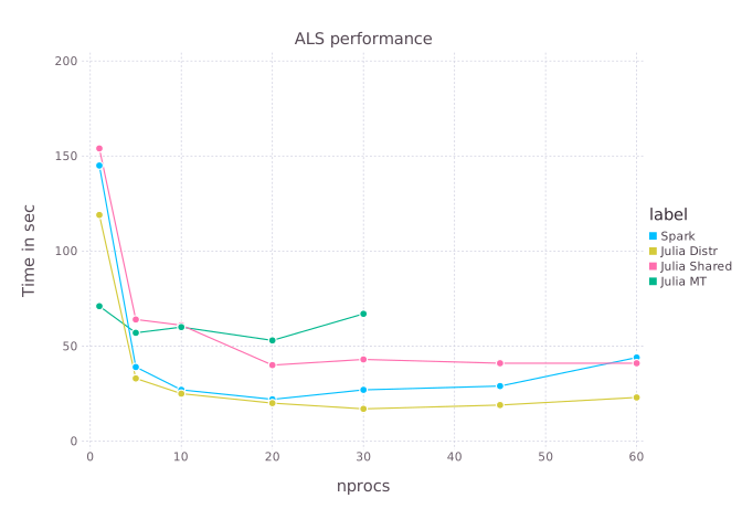
In the above graph, Julia Distr breaks up the problem and uses Julia’s distributed computing capabilities. Julia Shared uses shared memory through mmap arrays. Julia MT is the multithreading version of the ALS. While multi-threading in Julia is nascent, it already gives parallel speedups. There are several planned improvements to Julia’s multi-threading that we expect will make the multi-threaded ALS faster than the other parallel implementations.
The experiments were conducted by invoking spark with flags --master local[1]. The experiments were conducted on a 30 core Intel Xeon machine with 132 GB memory and 2 hyperthreads per core.
Credits to Tanmay KM for contributing towards the parallel implementation of the package.
Apart from methods to model the data and check for accuracy, there are also abilities to make recommendations for users who have not interacted with items, by picking the most likely items the user would interact with. Hence in RecSys.jl we have a fast, scalable and accurate recommender system which can be used to for end to end system. Currently we are working on a demo of such a recommender system with a UI interface too implemented in Julia.