Introduction

One of the most impressive features of Julia is that it lets you write generic code. Julia’s powerful LLVM-based compiler can automatically generate highly efficient machine code for base functions and user-written functions alike, on any architecture supported by LLVM, making you worry less about writing specialized code for each of these architectures.

One additional benefit of relying on the compiler for performance rather than hand-coding hot loops in assembly is that it is significantly more future proof. Whenever a next generation instruction set architecture comes out, your Julia code automatically gets faster.

Following a (very) brief look at what the hardware provides, we’ll look at a simple example (the sum function) to see how the compiler can take advantage of the hardware architecture to accelerate generic Julia functions.

Intel SIMD Hardware and Addition Instructions

Modern Intel chips provide a range of instruction set extensions. Among these are the various revisions of the Streaming SIMD Extension (SSE) and several generations of Advanced Vector Extensions (available with their latest processor families). These extensions provide Single Instruction Multiple Data (SIMD)-style programming, providing significant speed up for code amenable to such a programming style.

SIMD Registers are 128 (SSE), 256 (AVX) or 512 (AVX512) bits wide. They can generally be used in chunks of 8/16/32 or 64 bits, but exactly which divisions are available and which operations can be performed depend on the exact hardware achitecture.

Here is how the Add operation instructions on this architecture look like:

• (V)ADDPS: Takes two 128/256/512 bit values and adds 4/8/16 single precision values in parallel
• (V)ADDPD: Takes two 128/256/512 bit values and adds 2/4/8 double precision values in parallel
• (V)PADD(B/W/D/Q): Takes two 128/256/512 bit values and adds (up to 64) 8/16/32/64-bit integers in parallel
• (V)ADDSUBP(S,W): Takes two inputs, the operation is (+,-,+,-,…) on packed values
• There are also a few more exotic instructions that involve horizontal adds, saturating, etc.

An Example

The following code snippet shows a simple sum function (returning the sum of all the elements in an Array ‘a’) in Julia:

function mysum(a::Vector)
total = zero(eltype(a))
@simd for x in a				
total += x
end						
return total
end

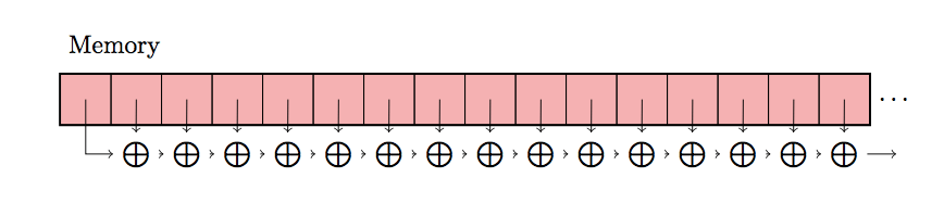
We can visualize this sequential operation, as a simple sequence of memory loads and additions:

However, this is not the code that Julia actually generates under the hood. By taking advantage of the SIMD instruction set, the add operation is performed in two phases:

1. During the first step (denoted “Vector Body” below), intermediate values are accumulated four at a time (in our example – depends on the hardware of course).

2. The reduction step, in which the final four elements are summed together.

This picture is simplified a bit, but conveys the general idea of the transformation, in the real code, there is a few extra caveats that the compiler has to pay attention to.

• If the array length is not known to be a multiple of the vector width, the compiler may have to generate an additional scalar part to sum the remaining elements (for high vector width – e.g. 32 that may itself use vector instructions). Depending on the hardware, the same is true if the memory alignment is not known.

• To take advantage of “superscalarness” (the ability of a processor to execute more than one instruction in parallel over and above SIMD), compilers will often “unroll” the vector body, keeping more than one SIMD register’s worth of state at the expense of a larger reduction step. (on the previous illustration, imagine the vector body copied four times vertically, with sums happening every fourth set of four values).

• If you’re summing floating-point, the above transformation may need to be explicitly allowed (the julia “@simd” macro does this for you), since floating-point arithmetic is in general non-associative (i.e. the result of the sum may differ between the two methods of computing it).

Machine Code Generated by the Compiler

In julia, we can use the @code_native macro to inspect the native code generated for any particular function. Trying this for our “mysum” function looks like for a summation of 100000 random numbers of Float64 type on a machine that supports AVX2, we can see precisely the pattern we expected:

@code_native mysum(rand(Float64 , 100000)) ;
vaddpd %ymm5, %ymm0, %ymm0
vaddpd %ymm6, %ymm2, %ymm2					
vaddpd %ymm7, %ymm3, %ymm3
vaddpd %ymm8, %ymm4, %ymm4
; NOTE: Omitting length check/branch here vaddpd %ymm0, %ymm2, %ymm0
vaddpd %ymm0, %ymm3, %ymm0
vaddpd %ymm0, %ymm4, %ymm0
vextractf128 $1, %ymm0, %xmm2
vaddpd %ymm2, %ymm0, %ymm0
vhaddpd %ymm0, %ymm0, %ymm0

The vector body phase on this machine is unrolled four times, using ymm0, 2, 3, and 4 as the accumulation registers.
The reduction step phase accumulates ymm2,3 and 4 into ymm0, and finally sums up parts of ymm0 itself to give the final result.

Here is how the machine code for the same function (arguments of type Float64) would look like on a machine that supports AVX512:

julia > @code_native mysum(rand(Float64 , 100000))  ;
vaddpd -192(%rdx), %zmm0, %zmm0
vaddpd -128(%rdx), %zmm2, %zmm2				
vaddpd -64(%rdx), %zmm3, %zmm3
vaddpd (%rdx), %zmm4, %zmm4
; NOTE: Omitting length check/branch here vaddpd %zmm0, %zmm2, %zmm0
vaddpd %zmm0, %zmm3, %zmm0
vaddpd %zmm0, %zmm4, %zmm0
vshuff64x2 $14, %zmm0, %zmm0, %zmm2 vaddpd %zmm2, %zmm0, %zmm0
vpermpd $238, %zmm0, %zmm2
vaddpd %zmm2, %zmm0, %zmm0
vpermilpd $1, %zmm0, %zmm2
vaddpd %zmm2, %zmm0, %zmm0

It is evident that the machine code generated might look different on other architectures, or with different data types, and might even look more complicated, but the pattern of generating the best machine code possible for Vector Body and Reduction phases on any architecture is consistent, therefore making auto-vectorization in Julia a cake walk.