By: n JuliaLang - The Julia programming language n
Re-posted from: https://julialang.org/blog/2021/01/precompile_tutorial/index.html
Tutorial on precompilation
By: n JuliaLang - The Julia programming language n
Re-posted from: https://julialang.org/blog/2021/01/precompile_tutorial/index.html
Tutorial on precompilation
By: Dean Markwick's Blog -- Julia
Re-posted from: https://dm13450.github.io/2021/01/01/Fundamental-AlphaVantage.html
AlphaVantage recently made fundamental data for stocks available through their
API and thanks to some new contributors to the AlphaVantage.jl Julia
package you can now easily import this data into your Julia project.
Enjoy these types of posts? Then sign up for my newsletter.
This fundamental data describes the underlying business information
about a company and is more fluid and open to interpretation than the
stock price. I’ll run through each of the new functions and try and
explain what data it returns.
The new data comes in through four different categories and functions:
plus a listing status to see what stocks are active.
The real value add though (if I do say so myself) comes from the
ability to pull out the annual or quarterly time series of a metric of
a stock easily and in a programatic manner. Using the metaprogramming
capabilities of Julia I was able to generate hundreds of functions
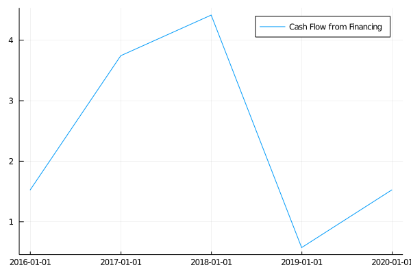
with just a for loop. Using these new functions you can now easily pull the quarterly revenue of Apple, cash flow from financing of Tesla or a timeseries of the current liabilities for Ford.
using AlphaVantage
using DataFrames, DataFramesMeta, Dates
using Plots
Firstly, we can get a list of stocks that are actively trading.
listingData = AlphaVantage.listing_status()
stocks = DataFrame(listingData[1], :auto)
rename!(stocks, Symbol.(vec(listingData[2])))
first(stocks, 5)
| symbol | name | exchange | assetType | ipoDate | delistingDate | |
|---|---|---|---|---|---|---|
| Any | Any | Any | Any | Any | Any | |
| 1 | A | Agilent Technologies Inc | NYSE | Stock | 1999-11-18 | null |
| 2 | AA | Alcoa Corp | NYSE | Stock | 2016-11-01 | null |
| 3 | AAA | AAF First Priority CLO Bond ETF | NYSE ARCA | ETF | 2020-09-09 | null |
| 4 | AAAU | Goldman Sachs Physical Gold ETF | NYSE ARCA | ETF | 2018-08-15 | null |
| 5 | AACG | ATA Inc | NASDAQ | Stock | 2008-01-29 | null |
Over 9000 stocks and ETF’s are listed. Which you can then do some simple sorting to look at the oldest listed stocks.
first(sort!(stocks, :ipoDate), 5)
| symbol | name | exchange | assetType | ipoDate | delistingDate | |
|---|---|---|---|---|---|---|
| Any | Any | Any | Any | Any | Any | |
| 1 | BA | Boeing Company | NYSE | Stock | 1962-01-02 | null |
| 2 | CAT | Caterpillar Inc | NYSE | Stock | 1962-01-02 | null |
| 3 | DD | DuPont de Nemours Inc | NYSE | Stock | 1962-01-02 | null |
| 4 | DIS | Walt Disney Co (The) | NYSE | Stock | 1962-01-02 | null |
| 5 | GE | General Electric Company | NYSE | Stock | 1962-01-02 | null |
When googling some of these stocks though, the IPO date doesn’t appear to be 100% correct. General Electric became a public company in 1896!
@where(stocks, :symbol .== "AAPL")
| symbol | name | exchange | assetType | ipoDate | delistingDate | status | |
|---|---|---|---|---|---|---|---|
| Any | Any | Any | Any | Any | Any | Any | |
| 1 | AAPL | Apple Inc | NASDAQ | Stock | 1980-12-12 | null | Active |
They have correctly recorded Apple’s IPO date though, so it might just
be something about older stocks, or something else I am missing.
The first new function is company_overview which does what it says
on the tin.
co = AlphaVantage.company_overview("AAPL", datatype = "json")
Dict{String,Any} with 59 entries:
  "SharesOutstanding"          => "17102499840"
  "ExDividendDate"             => "2020-11-06"
  "52WeekLow"                  => "52.8225"
  "ReturnOnEquityTTM"          => "0.7369"
  "LatestQuarter"              => "2020-09-30"
  "200DayMovingAverage"        => "111.2946"
  "EVToEBITDA"                 => "27.9399"
  "RevenuePerShareTTM"         => "15.82"
  "Beta"                       => "1.2976"
  "Sector"                     => "Technology"
  "ForwardAnnualDividendYield" => "0.0062"
  "Exchange"                   => "NASDAQ"
  "PercentInsiders"            => "0.066"
  "QuarterlyEarningsGrowthYOY" => "-0.023"
  "Currency"                   => "USD"
  "EBITDA"                     => "77343997952"
  "ShortRatio"                 => "1"
  "DividendYield"              => "0.0062"
  "AnalystTargetPrice"         => "127.11"
  "DilutedEPSTTM"              => "3.28"
  "BookValue"                  => "3.849"
  "LastSplitDate"              => "2020-08-31"
  "SharesFloat"                => "16984460162"
  "PriceToSalesRatioTTM"       => "8.4207"
  "FullTimeEmployees"          => "147000"
Here we get a dictionary with 59 different metrics about the company. There are lots of different quantitate and qualitative values about the company in question and provides a useful overview.
The income statement summarises a companies revenues and expenses. In short it shows where the money was coming in (revenue) and where it was going out (expenses).
is = AlphaVantage.income_statement("AAPL", datatype = "json")
Dict{String,Any} with 3 entries:
  "annualReports"    => Any[Dict{String,Any}("incomeTaxExpense"=>"9680000000","…
  "symbol"           => "AAPL"
  "quarterlyReports" => Any[Dict{String,Any}("incomeTaxExpense"=>"2228000000","…
Both the annual and quarterly results come back. For the annual reports there are the last 5 years. For the quarterly reports, the last 21 quarters.
keys(is["annualReports"][1])
Base.KeySet for a Dict{String,Any} with 29 entries. Keys:
  "incomeTaxExpense"
  "reportedCurrency"
  "otherNonOperatingIncome"
  "minorityInterest"
  "discontinuedOperations"
  "incomeBeforeTax"
  "totalOtherIncomeExpense"
  "interestIncome"
  "researchAndDevelopment"
  "grossProfit"
  "totalRevenue"
  "otherOperatingExpense"
  "taxProvision"
  "extraordinaryItems"
  "ebit"
  "otherItems"
  "netIncomeApplicableToCommonShares"
  "totalOperatingExpense"
  "costOfRevenue"
  "fiscalDateEnding"
  "interestExpense"
  "sellingGeneralAdministrative"
  "operatingIncome"
  "netIncomeFromContinuingOperations"
  "netIncome"
  ⋮
extrema(Date.(get.(is["annualReports"], "fiscalDateEnding", "")))
(Date("2016-09-30"), Date("2020-09-30"))
extrema(Date.(get.(is["quarterlyReports"], "fiscalDateEnding", "")))
(Date("2015-09-30"), Date("2020-09-30"))
Then what I have done is written the functions that allow you to extract any of the fields on a quarterly or annual basis. Which means you can easily plot some graphs and summarise the results.
totalRevenue = AlphaVantage.totalRevenue_quarterlys("AAPL", datatype =
"json")
plot(Date.(totalRevenue[:Date]),
     parse.(Float64, totalRevenue[:totalRevenue]) ./ 1e9,
     label = "Revenue (billions)",
     title = "Apple")
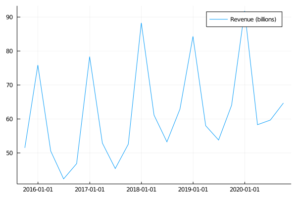
Here we have Apple quarterly total revenue, with a predictable pattern peaking in the first quarter.
A balance sheet summarises a companies assets, what it owns and its liabilities, what it owns to other people.
bs = AlphaVantage.balance_sheet("AAPL", datatype = "json")
Dict{String,Any} with 3 entries:
  "annualReports"    => Any[Dict{String,Any}("totalPermanentEquity"=>"None","wa…
  "symbol"           => "AAPL"
  "quarterlyReports" => Any[Dict{String,Any}("totalPermanentEquity"=>"None","wa…
string.(keys(bs["quarterlyReports"][1]))
51-element Array{String,1}:
 "totalPermanentEquity"
 "warrants"
 "negativeGoodwill"
 "preferredStockTotalEquity"
 "accumulatedAmortization"
 "inventory"
 "additionalPaidInCapital"
 "commonStockTotalEquity"
 "longTermInvestments"
 "fiscalDateEnding"
 "netTangibleAssets"
 "cashAndShortTermInvestments"
 "longTermDebt"
 ⋮
 "retainedEarnings"
 "shortTermInvestments"
 "propertyPlantEquipment"
 "goodwill"
 "preferredStockRedeemable"
 "totalLiabilities"
 "otherNonCurrentLiabilities"
 "currentLongTermDebt"
 "intangibleAssets"
 "accumulatedDepreciation"
 "otherCurrentLiabilities"
 "deferredLongTermAssetCharges"
Again, like the income statement, any of these keys can be extracted quarterly or annually.
fCash = AlphaVantage.cashAndShortTermInvestments_quarterlys("F",
datatype = "json")
fLiabilities = AlphaVantage.totalLiabilities_quarterlys("F", datatype
= "json")
cashPlot = plot(Date.(fCash[:Date]),
                parse.(Float64, fCash[:cashAndShortTermInvestments])/1e9,
                label="Cash and Short Term Investments (billions)",
                colour = "green")
liabPlot = plot(Date.(fLiabilities[:Date]),
                parse.(Float64, fLiabilities[:totalLiabilities])/1e9,
                label="Total Liabilities (billions)")
plot(cashPlot, liabPlot)
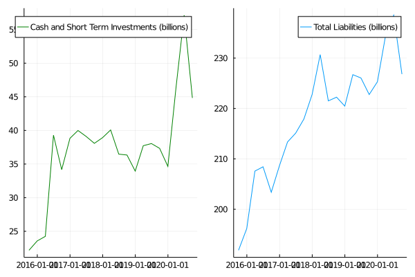
As per the intro I’ve plotted Fords cash and short term investment balance against something the owe, the total liabilities.
The cash flow statement shows the changes in the balance sheet. It helps judge a companies ability to meet its cash needs, i.e. pay their employers or service their debt.
cf = AlphaVantage.cash_flow("TSLA", datatype = "json")
Dict{String,Any} with 3 entries:
  "annualReports"    => Any[Dict{String,Any}("cashflowFromInvestment"=>"-428900…
  "symbol"           => "AAPL"
  "quarterlyReports" => Any[Dict{String,Any}("cashflowFromInvestment"=>"5531000…
string.(keys(cf["quarterlyReports"][1]))
24-element Array{String,1}:
 "cashflowFromInvestment"
 "changeInInventory"
 "reportedCurrency"
 "changeInAccountReceivables"
 "changeInCashAndCashEquivalents"
 "otherOperatingCashflow"
 "dividendPayout"
 "changeInReceivables"
 "capitalExpenditures"
 "changeInExchangeRate"
 "operatingCashflow"
 "cashflowFromFinancing"
 "changeInLiabilities"
 "stockSaleAndPurchase"
 "otherCashflowFromFinancing"
 "changeInOperatingActivities"
 "depreciation"
 "fiscalDateEnding"
 "changeInCash"
 "netBorrowings"
 "investments"
 "netIncome"
 "changeInNetIncome"
 "otherCashflowFromInvestment"
cashflow = AlphaVantage.cashflowFromFinancing_annuals("TSLA", datatype="json")

plot(Date.(cashflow[:Date]),
     parse.(Float64, cashflow[:cashflowFromFinancing]) ./ 1e9,
     label="Cash Flow from Financing (billions)",
     title = "Tesla")
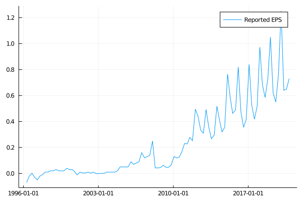
Each company reports their earnings each quarter and summarise their performance of the previous quarter. There are more dates available for earnings, but also slightly different fields for the quarterly and annual results.
earnings = AlphaVantage.earnings("AAPL", datatype = "json")
Dict{String,Any} with 3 entries:
  "annualEarnings"    => Any[Dict{String,Any}("fiscalDateEnding"=>"2020-09-30",…
  "quarterlyEarnings" => Any[Dict{String,Any}("reportedDate"=>"2020-10-29","est…
  "symbol"            => "AAPL"
string.(keys(earnings["annualEarnings"][1]))
2-element Array{String,1}:
 "fiscalDateEnding"
 "reportedEPS"
string.(keys(earnings["quarterlyEarnings"][1]))
6-element Array{String,1}:
 "reportedDate"
 "estimatedEPS"
 "surprise"
 "surprisePercentage"
 "fiscalDateEnding"
 "reportedEPS"
extrema(Date.(get.(earnings["quarterlyEarnings"], "reportedDate", "")))
(Date("1996-04-17"), Date("2020-10-29"))
extrema(Date.(get.(earnings["annualEarnings"], "fiscalDateEnding", "")))
(Date("1996-09-30"), Date("2020-09-30"))
reported = AlphaVantage.reportedEPS_quarterlyEarnings("AAPL",
datatype="json")
plot(Date.(reported[:Date]),
     parse.(Float64, reported[:reportedEPS]),
     label="Reported EPS",
     title = "Apple")
There you go, lots more functions for the package and something
different than just looking at stock prices. This fundamental data
adds another dimension to any quantitate analysis of different stocks
so go grab your free API key from
AlphaVantage and get exploring!
If you are new to AlphaVantage you can also check out my previous post
on getting market data into Julia.
Re-posted from: https://bkamins.github.io/julialang/2020/12/31/randu.html
Today finally the Train Your Brain book by Paweł Prałat and me is finally
available. In the book we argue that using computer support can help solve
mathematical problems.
In this post I thought of doing the reverse — consider a classical computing
problem that can be better understood using mathematics. Here I concentrate on
the computational part, but all the theory needed to rigorously study what I
discuss is presented in the Train Your Brain book.
The topic I want to tackle today is why devising a good pseudo random number
generator is hard. I will use the classical RANDU generator to
highlight potential problems that one might encounter in practice.
This post was tested under Julia 1.5.3, DataFrames.jl 0.22.2, FreqTables.jl
0.4.2, HypothesisTests.jl 0.10.2, Pipe.jl 1.3.0, and PyPlot.jl 2.9.0.
As a warning note that some of the computations we do in this post can take up
to several minutes and require at least several GB of RAM (I used @time to
highlight the most expensive steps), so if you run my code you should take this
into account.
Let us get started!
The RANDU generator produces floating point values from the \((0,1)\)
interval using the following rule. Let \(S_i\) be the state of the generator
at time \(i\). Then is next state is defined as:
\[S_{i+1}=65539S_i \mod 2^{31},\]
and the produced float value is \(S_{i+1} / 2^{31}\).
We start with loading the libraries we will use in this Julia session:
using DataFrames
using FreqTables
using HypothesisTests
using Pipe
using PyPlot
using Random
using Statistics
Now implement the RANDU generator:
const RANDU_CONST = 0x00010003

mutable struct Randu <: AbstractRNG
    state::UInt32
end

Random.seed!(r::Randu, state::UInt32) = (r.state = state; return r)
Base.copy(r::Randu) = Randu(r.state)

function Random.rand(r::Randu,
                     ::Random.SamplerTrivial{Random.CloseOpen01{Float64}})
    s = r.state
    s = (s * RANDU_CONST) & 0x7fffffff
    r.state = s
    return s / 0x80000000
end
Observe that we use UInt32 for all computations and as \(2^{31}\) is a divisor
of \(2^{32}\) we can safely ignore the overflow – we simply look at the lowest
31 bits of the generated numbers, which is done by performing the & 0x7fffffff
operation.
Now we are ready to get started with using this generator to produce Float64
pseudo random values from the \((0,1)\) range.
First we want to produce random permutations using the generator. Here is
the code that counts how many distinct permutations we get if the length
of the permutation is 64 and we produce 10,000,000 of them.
count_permutations(rng::AbstractRNG) =
    mapreduce(push!, 1:10_000_000, init=Set{Vector{Int}}()) do _
        sortperm(rand(rng, 64))
    end |> length
Let us start with using MersenneTwister that is currently used as a default
generator in Julia:
julia> @time count_permutations(MersenneTwister(11))
 64.585667 seconds (30.11 M allocations: 12.058 GiB, 34.31% gc time)
10000000
We can see that we got no duplicates. Now let us test our RANDU generator:
julia> @time count_permutations(Randu(11))
 61.817341 seconds (30.00 M allocations: 12.052 GiB, 31.82% gc time)
8388608

julia> @time count_permutations(Randu(12))
 39.189380 seconds (30.00 M allocations: 11.841 GiB, 19.51% gc time)
2097152
Now we got many duplicates, and we see that 12 produced many more than 11.
Let us start with trying to understand what we should expect in this case. We
have \(64!\) permutations (buckets) and \(10^7\) values so the probability
of not seeing any duplicate is:
\[1 – \prod_{i=0}^{10^7-1}\left(1-\frac{i}{64!}\right)\]
This value can be approximated from above by (where the above formula comes from
and how to do such approximations is explained in our book):
\[1 – \exp\left(-\frac{10^7\cdot (10^7-1)}{2\cdot 64!-10^7}\right)\]
This can be easily computed using Julia:
julia> Float64(1 - exp(-10_000_000*(10_000_000-1)/
                       (2*(factorial(big(64))-10_000_000))))
3.9726375353434445e-76
As you can see the probability of seeing any duplicate is extremely low,
so there must be some flaw in the RANDU generator.
In this case the problem is that it does not produce enough randomness. We can
see that the generator has at most \(2^{31}\) states (actually it has less as we
will find out soon) and it seems not enough for our purposes.
Let us investigate it in more detail. Let us first check for what smallest
positive \(c\) we have:
\[65539^c \equiv 1 \mod (2^{31})\]
as then we will have that
\[S_1 \equiv S_{c+1} \mod (2^{31})\]
and thus get a cycle. Here is the code:
julia> function find_min_power()
         m = RANDU_CONST
         i = one(UInt32)
         while m & 0x7fffffff != 1
             m *= RANDU_CONST
             i += one(UInt32)
         end
         return i
       end
find_min_power (generic function with 1 method)

julia> find_min_power()
0x20000000

julia> RANDU_CONST^0x20000000 & 0x7fffffff
0x00000001
and we see that \(c=2^{29}\) (again why it is \(2^{29}\) and how it could have
been computed using pen and paper is explained in our book). This means
that given any starting seed \(S_1\) we cannot generate more than \(2^{29}\)
distinct values. This is not much indeed for current computing standards.
However, let us investigate why seed 12 was much worse than seed 11. Here is the
code:
julia> function get_cycles()
           cycle = zeros(UInt8, 0x80000000)
           c = 0x1
           for k in 1:2^31-1
               i = k
               cycle[i] != 0x0 && continue
               while cycle[i] == 0x0
                   cycle[i] = c
                   i = (i * RANDU_CONST) & 0x7fffffff
               end
               @assert i == k # we should get a cycle
               c += 0x1
               @assert c != 0x0 # make sure we do not have more than 255 cycles
           end
           return cycle
       end
get_cycles (generic function with 1 method)

julia> @time cycle = get_cycles()
127.491600 seconds (2 allocations: 2.000 GiB, 0.29% gc time)
2147483648-element Array{UInt8,1}:
 0x01
 0x02
 0x01
 0x03
 0x04
 0x02
 0x04
 0x05
 0x01
 0x06
    ⋮
 0x0a
 0x01
 0x06
 0x01
 0x08
 0x04
 0x06
 0x04
 0x00

julia> freq_cycle = sort(freqtable(cycle), rev=true)
61-element Named Array{Int64,1}
Dim1  │
──────┼──────────
0x01  │ 536870912
0x04  │ 536870912
0x02  │ 268435456
0x06  │ 268435456
0x03  │ 134217728
0x08  │ 134217728
0x05  │  67108864
0x0a  │  67108864
0x07  │  33554432
⋮               ⋮
0x33  │         8
0x38  │         8
0x35  │         4
0x3a  │         4
0x37  │         2
0x39  │         2
0x3c  │         2
0x00  │         1
0x3b  │         1

julia> freqtable(freq_cycle)
30-element Named Array{Int64,1}
Dim1      │
──────────┼──
1         │ 2
2         │ 3
4         │ 2
8         │ 2
16        │ 2
32        │ 2
64        │ 2
128       │ 2
256       │ 2
⋮           ⋮
2097152   │ 2
4194304   │ 2
8388608   │ 2
16777216  │ 2
33554432  │ 2
67108864  │ 2
134217728 │ 2
268435456 │ 2
536870912 │ 2
And we see that we have two cycles having \(2^{29}\) length and many shorter
cycles. The shortest one has length 1, let us check if this is indeed the case:
julia> x = UInt32(only(findall(==(0x3b), cycle)))
0x40000000

julia> x * RANDU_CONST & 0x7fffffff
0x40000000
So if we are unlucky with the choice of the initial seed we will get the cycle
of length 1. This phenomenon is called a bad seed problem in pseudo random
number generators. However, a cursory look at cycle variable suggests that
it is the case that all odd numbers are good seeds (producing cycle of length
\(2^{29}\)). Let us check this:
julia> foreach(enumerate(cycle)) do (i, v)
           @assert iseven(i) ⊻ (v == 0x1 || v == 0x4)
       end

julia>
We got no error so indeed this the case. Actually the two longest cycles contain
two groups of odd numbers that respectively are congruent to 1 and 3, or 5 and 7
modulo 8 as we can see here:
julia> ([1, 3, 5, 7] .* RANDU_CONST) .% 8
4-element Array{Int64,1}:
 3
 1
 7
 5
This, in particular, shows us that low bits of the generated numbers show a
pattern so RANDU is not well suited for generation of integers. But maybe it
is good when generating floats?
Before checking this let me just summarize that we have up to this point learned
that if we use a good (i.e. odd) seed we have a generator that has a cycle of
\(2^{29}\). This means that it is essentially only useful if we generate very few
random numbers by todays standards. Above we saw that this causes a problem when
generating permutations. Before we move on let us check out another scenario of
generating binary numbers:
julia> function gen2(rng::AbstractRNG)
           means = Float64[]
           for _ in 1:1000
               s = 0
               for _ in 1:10^8
                   s += rand(rng) < 0.5
               end
               push!(means, s / 10^8)
           end
           return var(means), quantile([var(rand(means, 1000)) for _ in 1:10000],
                                       [0.025, 0.975])
       end
gen2 (generic function with 1 method)

julia> @time gen2(Randu(11))
124.834623 seconds (10.02 k allocations: 77.684 MiB)
(3.806128771508955e-9, [3.540403887824998e-9, 4.062688436887708e-9])

julia> 0.25 / 10^8 # we should get approximately this value
2.5e-9
and we can see that the variance produced for \(10^8\) trials is much to large
(note that doing 1000 repetitions of the experiment ensured that the differences
are significant, which we checked using bootstrapping). Conversely, we could
have easily made the variance too small if we use e.g. \(2^{29}\) trials (as you
can see below we got exactly the same value 100 times — for sure not producing
enough variance):
julia> function gen2_v2(rng::AbstractRNG)
           means = Float64[]
           for _ in 1:100
               s = 0
               for _ in 1:2^29
                   s += rand(rng) < 0.5
               end
               push!(means, s / 2^29)
           end
           return freqtable(means)
       end
gen2_v2 (generic function with 1 method)

julia> @time gen2_v2(Randu(11))
 62.797411 seconds (42 allocations: 5.156 KiB)
1-element Named Array{Int64,1}
Dim1  │
──────┼────
0.5   │ 100
Have a look two plots that were generated using this code:
function plot_square(rng::AbstractRNG)
    v = Tuple{Float64, Float64}[]
    for i in 1:2^28
        x, y = rand(rng), rand(rng)
        if 0.4 < x < 0.401 && 0.5 < y < 0.501
            push!(v, (x,y))
        end
    end
    scatter(getindex.(v, 1), getindex.(v, 2), s=1)
end
Here are the plots:
plot_square(Randu(11))

plot_square(MersenneTwister(11))

The RANDU plot looks oddly regular. The points seem to lie on parallel lines.
It is clear that \(S_{i+1} / 2^{31} – 65539\cdot S_{i} / 2^{31}\) is an integer
as \(S_{i+1}=65539S_i \mod 2^{31}\). However, if we had only this relationship
would not get the pattern we see above. Let us look for other lines of this type
(we limit ourselves to small values of pairs defining the lines):
julia> function find_2d()
           for a in 1:RANDU_CONST
               b = a * RANDU_CONST & 0x7fffffff
               a + b <= RANDU_CONST + 1 && @show a, -b
               b = 0x80000000 - b
               a + b <= RANDU_CONST + 1 && @show a, b
           end
       end
find_2d (generic function with 1 method)

julia> find_2d()
(a, -b) = (1, -65539)
(a, b) = (32766, 32774)
(a, -b) = (32767, -32765)
Now, of the two pairs (32766, 32774) and (32767, -32765) which one can be
expected to produce bigger spacing between the lines? Note that both produce
values in the similar width of the range. However, (32766, 32774) produces
only odd values (as we assume to use odd seed value), while (32767, -32765)
produces both even and odd values because:
\[a\frac{S_{i+1}}{2^{31}}+b\frac{S_i}{2^{31}} =
\frac{a (65539 S_i \mod 2^{31})}{2^{31}}+\frac{b S_i}{2^{31}} =
\frac{a (65539 S_i + 2^{31}p)}{2^{31}}+\frac{b S_i}{2^{31}}\]
where \(p\) is an integer, and after rearranging we get:
\[\frac{(65539a+b) S_i + 2^{31}ap}{2^{31}}\]
Now for both our \((a, b)\) pairs we have that \(65539a+b=2^{31}\) so it reduces
to:
\[S_i+ap.\]
Since \(S_i\) is odd, we see that for \(a=32766\) this is always an odd number,
while for \(a=32767\) it can be either even or odd number as discussed.
So for (32766, 32774) we expect to get \((32766+32774)/2= 32770\) distinct
integer values. Let us check this:
julia> let ru = Randu(11), s = Set{Int}()
           for _ in 1:2^28
               v = Int(32774*rand(ru)+32766*rand(ru))
               @assert isodd(v)
               push!(s, v)
           end
           length(s)
       end
32770
Having 32700 parallel lines on which the points lie is bad (we can see this
above), but probably not prohibitive. The real problem starts when we look
at the triplets of points and check if we can put them on a few planes
(again we limit ourselves to only small values of pairs defining the lines):
julia> function find_3d()
           a = 1
           for b in 0:RANDU_CONST, signb in [-1, 1]
               c = (a * RANDU_CONST^2 + signb * b * RANDU_CONST) & 0x7fffffff
               a + b + c <= RANDU_CONST && @show a, signb*b, -c
               c = 0x80000000 - c
               a + b + c <= RANDU_CONST && @show a, signb*b, c
           end
       end
find_3d (generic function with 1 method)

julia> find_3d()
(a, signb * b, -c) = (1, -5, -65530)
(a, signb * b, c) = (1, -6, 9)
(a, signb * b, -c) = (1, 32761, -32756)
(a, signb * b, -c) = (1, -32772, -32765)
Bam – we got a very bad (1, -6, 9) tuple! Now we understand the reason for
the famous RANDU plot that you can see in Wikipedia artice I linked
above:

Before we move on let us check the same with our code:
julia> let ru = Randu(11), s = Set{Int}()
           for _ in 1:ceil(Int, 2^29 / 3)
               push!(s, 9*rand(ru) - 6*rand(ru) + rand(ru))
           end
           length(s)
       end
15
But why it is a problem? Let us illustrate it by splitting each of three
dimensions into \(16\) bins (so we get \(16^3\) bins in total). Finally we use
the DataFrames.jl package (which I assume everyone was waiting for :), as it was
announced in the introduction and every story teller tries to follow Чеховское
ружьё principle):
julia> @time res3d = let
           df = DataFrame(x1=UInt8[], x2=UInt8[], x3=UInt8[])
           ru = Randu(11)
           for _ in 1:ceil(Int, 2^29 / 3)
               push!(df, trunc.(UInt8, 16 .* (rand(ru), rand(ru), rand(ru))))
           end
           df
       end
 52.469085 seconds (1.25 G allocations: 18.675 GiB, 3.29% gc time)
178956971×3 DataFrame
       Row │ x1     x2     x3
           │ UInt8  UInt8  UInt8
───────────┼─────────────────────
         1 │     0      0      0
         2 │     0      2      7
         3 │    11     13     13
         4 │     1      0      9
         5 │     3     14      3
         6 │     8      2     14
         7 │     2     15      5
     ⋮     │   ⋮      ⋮      ⋮
 178956965 │     4      5      3
 178956966 │     4     12      0
 178956967 │    15      8     11
 178956968 │     6     11     11
 178956969 │    15     10     15
 178956970 │    15      3      6
 178956971 │     7      0      0
           178956957 rows omitted

julia> @time agg3d = @pipe res3d |>
                     groupby(_, [:x1, :x2, :x3]) |>
                     combine(_, nrow) |>
                     sort(_, :nrow, rev=true)
  5.939132 seconds (216 allocations: 4.667 GiB, 0.78% gc time)
3840×4 DataFrame
  Row │ x1     x2     x3     nrow
      │ UInt8  UInt8  UInt8  Int64
──────┼────────────────────────────
    1 │     5      1      7  78360
    2 │     6      7      3  78300
    3 │     3     12     12  78268
    4 │     7     13     12  78215
    5 │     2      5     11  78201
    6 │     0      2      9  78201
    7 │     5      2     13  78199
  ⋮   │   ⋮      ⋮      ⋮      ⋮
 3834 │    10      2      9   6339
 3835 │    12     15      3   6336
 3836 │    10      0     13   6332
 3837 │    11      3      4   6331
 3838 │     7      3      8   6329
 3839 │     6      3      3   6313
 3840 │     3      0     12   6299
                  3826 rows omitted

julia> nrow(agg3d), 16^3
(3840, 4096)

julia> nrow(res3d) / 16^3
43690.666748046875
What do we see here. We used a bit over \(2^{29}\) random numbers (so we went
through the whole cycle of the generator). We got 3840 non-empty bins out of a
total of 4096 possible bins. Also we can see that as the average bin size is
around 43691 we have bins that are almost twice as populated and bins that
contain very small number of values. An extremely unlikely situation as we can
see with this test:
julia> bins = zeros(Int, 16^3);

julia> copyto!(bins, agg3d.nrow);

julia> pvalue(ChisqTest(bins))
0.0
The reason is obvious – we have points lying on fifteen planes and using
\(16\times16\times16\) grid we are very often hitting the holes between the
planes (which also means that to balance this sometimes we are hitting overly
dense regions of points by other bins). This clearly shows that using RANDU to
perform e.g. integration using MonteCarlo simulation in higher dimensions is not
advisable.
Let us give a simple example of this. We want to integrate a function:
\[f(\mathbf(x)) = 20^n \exp\left(-20\sum_{i=1}^nx_i\right),\]
where \(n\) is a number of dimensions and will range from \(1\) to \(4\).
We want to calculate its integral over \([0,1]^n\). Analytically we know it is
equal to \((1-\exp(-20))^n\), so it is almost \(1\).
Let us check the results:
julia> let ru = Randu(111)
       for n in 1:4
           int = mean(f(rand(ru, n)) for _ in 1:10^8)
           @show n, int
       end
       end
(n, int) = (1, 0.9999974000942274)
(n, int) = (2, 1.0002307988280261)
(n, int) = (3, 1.3654740670592842)
(n, int) = (4, 2.355245785641749)
Note how bad it becomes in dimension higher than 2 (I omit testing statistical
significance of the deviation for \(10^8\) samples and encourage you to perform
it as an exercise).
We can compare it to MersenneTwister results:
julia> let mt = MersenneTwister(111)
       for n in 1:4
           int = mean(f(rand(mt, n)) for _ in 1:10^8)
           @show n, int
       end
       end
(n, int) = (1, 0.9994916961823186)
(n, int) = (2, 1.000145832437786)
(n, int) = (3, 0.9932430835430406)
(n, int) = (4, 0.9993585894631343)
which produces following what would normally be expected.
I hope this post highlighted typical problems the pseudo random number
generators may posses, and the practical consequences of these issues. I also
tried to show how nicely such an analysis can be performed using the Julia
language and the packages from the JuliaData ecosystem.
I encourage you to play around with different pseudo random number generators
and check if they pass or fail the tests I have presented. If you want to learn
more about testing pseudo random number generators then this article
is a good place to start.
Happy New Year!