Tag Archives: Julia

How to (Almost) Never Lose A Game

By: Alec Loudenback

Re-posted from: https://alecloudenback.com/posts/counting-chickens/index.html

Count Your Chickens is a cooperative game for children. I have very much enjoyed playing it with my daughter but an odd pattern appeared across many attempts: we never lost.

The game is entirely luck-based and is fairly straightforward. There are a bunch of chicks out of the chicken coop, and as you move from one space to another, you collect and return the chicks to the coop based on how many spaces you moved. You simply spin a spinner and move to the next icon that matches what you spun. There are some bonus spaces (in blue) where you get to collect an extra chick and you can also spin a fox which removes a chick from the coop.

I had a suspicion that if you were missing chicks from the game, that the game would quickly become much easier to “win” by getting all of the chicks back into the coop. Simultaneously, I had learned about SumTypes.jl and wanted to try it out. So could we simulate the game by using enumerated types? Yes, and here’s how it worked:

Setup

We’ll use four packages:

1using SumTypes
2using CairoMakie
3using ColorSchemes
4using DataFramesMeta
1
Used to model the different types of squares.
2
We’ll use this to plot outcomes of games.
3
To show the distribution of outcomes, we’ll use a custom color set for the plot.
4
Dataframe manipulation will help transform our simulated results for plotting.

Sum Types

What they are is nicely summarized as:

Sum types, sometimes called ‘tagged unions’ are the type system equivalent of the disjoint union operation (which is not a union in the traditional sense). In the Rust programming language, these are called “Enums”, and they’re more general than what Julia calls an enum.

At the end of the day, a sum type is really just a fancy word for a container that can store data of a few different, pre-declared types and is labeled by how it was instantiated.

Users of statically typed programming languages often prefer Sum types to unions because it makes type checking easier. In a dynamic language like Julia, the benefit of these objects is less obvious, but there are cases where they’re helpful, like performance sensitive branching on heterogeneous types, and enforcing the handling of cases.

We have two sets of things in this game which are similar and candidates for SumTypes:

  1. The animals on the spinner, and
  2. The different types of squares on the board.

It’s fairly simple for Animal, but Square needs a little explanation:

"Animal resprents the type of creature on the spinner and board."
@sum_type Animal begin
    Cow
    Tractor
    Sheep
    Dog
    Pig
    Fox
end

"""
Square represents the three different kinds of squares, including regular and bonus squares that contain data indicating the `Animal` in the square.
"""
@sum_type Square begin
    Empty
1    Regular(::Animal)
    Bonus(::Animal)
end
1
@sum_type will create variants that are all of the same type (Square in this case). The syntax Regular(::Animal) indicates that when, e.g, we create a Regular(Dog) we will get a Square that encloses data indicating it’s both a Regular variant of a Square in addition to holding the Dog instance of an Animal. That is, Regular(Dog) is an instance of Square type and does not create a distinct subtype of Square.

A couple of examples to show how this works:

typeof(Pig), Pig isa Animal
(Animal, true)
typeof(Bonus(Dog)), Bonus(Dog) isa Square
(Square, true)

Game Logic

I’ll first define a function that outlines how the game works and allow the number of chicks in play to vary since that’s the thesis for why it might be easier to win with missing pieces. Then I define two helper functions which give us the right behavior depending on the result of the spinner and the current state of the board. They are described in the docstrings.

"""
    playgame(board,total_chicks=40)

Simulate a game of Count Your Chickens and return how many chicks are outside of the coop at the end. The players win if there are no chicks outside of the coop. 
"""
function playgame(board, total_chicks=40)
    position = 0
    chicks_in_coop = 0
    while position < length(board)
        spin = rand((Cow, Tractor, Sheep, Dog, Pig, Fox))
        if spin == Fox
            if chicks_in_coop > 1
                chicks_in_coop -= 1
            end
        else
            result = move(board, position, spin)
            # limit the chicks in coop to available chicks remaining
            moved_chicks = min(total_chicks - chicks_in_coop, result.chicks)
            chicks_in_coop += moved_chicks
            position += result.spaces
        end
    end
    return total_chicks - chicks_in_coop

end
"""
    move(board,cur_position,spin)

Represents the result of a single turn of the game. 
Returns a named pair (tuple) of the number of spaces moved and chicks collected for that turn. 
"""
function move(board, cur_position, spin)
    next_square = findnext(space -> ismatch(space, spin), board, max(cur_position, 1))

    if isnothing(next_square)
        # nothing found that matches, so we must be at the end of the board
        l = length(board) - cur_position + 1
        (spaces=l, chicks=l)
    else
        n_spaces = next_square - cur_position
1        @cases board[next_square] begin
            Empty => (spaces=n_spaces, chicks=n_spaces)
            Bonus => (spaces=n_spaces, chicks=n_spaces + 1)
            Regular => (spaces=n_spaces, chicks=n_spaces)
        end
    end
end
1
SumTypes.jl provides a way to match the value of the board at the next square to Empty (which shouldn’t actually happen), Bonus, or Regular and the result depends on which kind of board we landed on.
"""
    ismatch(space,spin)

True or false depending on if the `spin` (an `Anmial`) matches the data within the `square` (`Animal` if not an `Empty` `Square`). 
"""
function ismatch(square, spin)
    @cases square begin
        Empty => false
1        [Regular, Bonus](a) => spin == a
    end
end
1
The [...] lets us simplify repeated cases while the (a) syntax allows us to reference the encapsulated data within the Square SumType.

Last part of the setup is declaring what the board looks like (unhide if you want to see – it’s just a long array representing each square on the board):

Code
board = [
    Empty,
    Regular(Sheep),
    Regular(Pig),
    Bonus(Tractor),
    Regular(Cow),
    Regular(Dog),
    Regular(Pig),
    Bonus(Cow),
    Regular(Dog),
    Regular(Sheep),
    Regular(Tractor),
    Empty,
    Regular(Cow),
    Regular(Pig),
    Empty,
    Empty,
    Empty,
    Regular(Tractor),
    Empty,
    Regular(Tractor),
    Regular(Dog),
    Bonus(Sheep),
    Regular(Cow),
    Regular(Dog),
    Regular(Pig),
    Regular(Tractor),
    Empty,
    Regular(Sheep),
    Regular(Cow),
    Empty,
    Empty,
    Regular(Tractor),
    Regular(Pig),
    Regular(Sheep),
    Bonus(Dog),
    Empty,
    Regular(Sheep),
    Regular(Cow),
    Bonus(Pig),]

Examples

Here are a couple examples of how the above works. First, here’s an example where we check if our spin (a Pig matches a candidate square Bonus(Pig)):

ismatch(Bonus(Pig), Pig)
true

If our first spin was a Pig, then we would move 3 spaces and collect 3 chicks:

move(board, 0, Pig)
(spaces = 3, chicks = 3)

And a simulation of a game:

playgame(board, 40)
0

Game Dynmaics

To understand the dynamics, we will simulate 1000 games for each variation of chicks from 35 (less than should come with the game) to 42 (more than should come with the game).

chick_range = 35:42
n = 1000
n_chicks = repeat(chick_range, n)
outcomes = playgame.(Ref(board), n_chicks)

df = DataFrame(; n_chicks, outcomes)


df = @chain df begin
    # create a wide table with the first column being the 
    # number of remaining chicks while the others 
    # total chicks
    unstack(:outcomes, :n_chicks, :outcomes, combine=length)
    # turn the missing values into 0 times this combination occurred
    coalesce.(_, 0)
    # # calculate proportion of outcomes within each column
    transform(Not(:outcomes) .=> x -> x / sum(x), renamecols=false)
    # restack back into a long table
    stack(Not(:outcomes))
end
# parse the column names which became strings when unstacked to column name
df.n_chicks = parse.(Int, df.variable)
df
104×4 DataFrame
79 rows omitted
Row outcomes variable value n_chicks
Int64 String Float64 Int64
1 0 35 0.986 35
2 2 35 0.004 35
3 1 35 0.01 35
4 5 35 0.0 35
5 3 35 0.0 35
6 6 35 0.0 35
7 4 35 0.0 35
8 7 35 0.0 35
9 8 35 0.0 35
10 14 35 0.0 35
11 11 35 0.0 35
12 9 35 0.0 35
13 10 35 0.0 35
93 2 42 0.22 42
94 1 42 0.186 42
95 5 42 0.07 42
96 3 42 0.188 42
97 6 42 0.028 42
98 4 42 0.113 42
99 7 42 0.011 42
100 8 42 0.01 42
101 14 42 0.001 42
102 11 42 0.001 42
103 9 42 0.002 42
104 10 42 0.0 42

Now to visualize the results, we want to create a custom color scheme where the color is green if we “win” and an increasingly intense red color the further we were from winning the game (not all chicks made it back to the coop).

colors = vcat(get(ColorSchemes.rainbow, 0.5), get.(Ref(ColorSchemes.Reds_9), 0.6:0.025:1.0))

let
    f = Figure()
    ax = Axis(f[1, 1],
        title="Count Your Chickens Win Rate",
        xticks=chick_range,
        xlabel="Number of chicks",
        ylabel="Proportion of games",
    )
    bp = barplot!(df.n_chicks, df.value,
        stack=df.outcomes,
        color=colors[df.outcomes.+1],
        label=df.outcomes,
    )

    f
end
┌ Warning: Found `resolution` in the theme when creating a `Scene`. The `resolution` keyword for `Scene`s and `Figure`s has been deprecated. Use `Figure(; size = ...` or `Scene(; size = ...)` instead, which better reflects that this is a unitless size and not a pixel resolution. The key could also come from `set_theme!` calls or related theming functions.
└ @ Makie ~/.julia/packages/Makie/fyNiH/src/scenes.jl:220
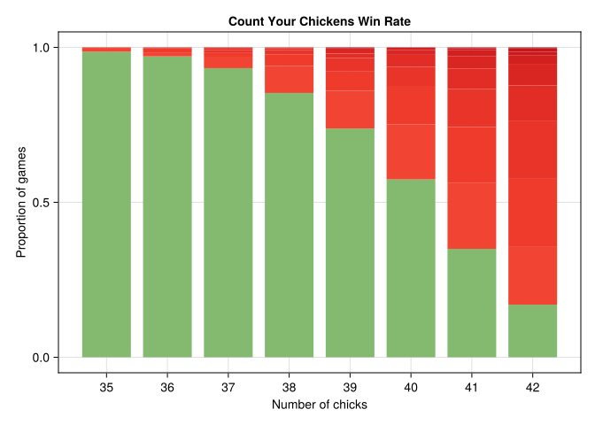
We can see that if we have 40 chicks (probably by design) we’d expect to win just over 50% of the time (which is less often that I would have guessed for the game’s family friendly approach).

However, if you were missing a few pieces like we were, your probability of winning dramatically increases and explains our family’s winning streak.

Endnotes

Environment

Julia Packages:

using Pkg;
Pkg.status();
Status `~/prog/alecloudenback.com/posts/counting-chickens/Project.toml`
  [13f3f980] CairoMakie v0.11.5
  [35d6a980] ColorSchemes v3.24.0
  [1313f7d8] DataFramesMeta v0.14.1
  [8e1ec7a9] SumTypes v0.5.5

Acknowledgements

Thanks to Mason Protter who provided some clarifications on the workings of SumTypes.jl.

ChatGPT performs better on Julia than Python (and R) for Large Language Model (LLM) Code Generation. Why?

By: Christopher Rackauckas

Re-posted from: http://www.stochasticlifestyle.com/chatgpt-performs-better-on-julia-than-python-and-r-for-large-language-model-llm-code-generation-why/

Machine learning is all about examples. The more data you have, the better it should perform, right? With the rise of ChatGPT and Large Language Models (LLMs) as a code helping tool, it was thus just an assumption that the most popular languages like Python would likely be the best for LLMs. But because of the increased productivity, I tend to use a lot of Julia, a language with an estimated user-base of around a million programmers. For this reason, people have often asked me how it fairs with ChatGPT, Github Copilot, etc., and so I checked out those pieces and… was stunned. It’s really good. It seemed better than Python actually?

The data is in: Julia does well with ChatGPT

This question was recently put to the test by a researcher named Alessio Buscemi in A Comparative Study of Code Generation using ChatGPT 3.5 across 10 Programming Languages. Basically, he setup a bunch of example problems and asked ChatGPT for the code, executed it, and documented the results. The main result of the paper is the following:

or in the words of the author:

“Overall, 1833 runs, or 45.8% of the total number, lead to executable code. However, this percentage varies greatly according to the tested language. ChatGTP performs the best on Julia, with a 81.5% of generated code being successfully executed, and performs the worst on C++, with only 7.3% of the executions being successful. Specifically, the model seems to perform better on high-level dynamically typed languages (Javascript, Julia, Perl, Python, R, Ruby, Smalltalk) rather than lower level statically typed languages (C, C++, Go).”

That is right, of all languages, “ChatGTP performs the best on Julia”. In fact, ChatGPT generally only performs well on slow languages: Julia is the only fast language that it did well on. The author went on to do a podcast at DataSkeptic where at 25:20 this is addressed where he was unable to answer why ChatGPT was able to make him more successful in Julia than Python, even though he himself only had used Python before.

Is it unexpected that Julia would outperform Python in generated code execution and correctness?

But the real question is, is this really unexpected? I don’t think so, this aligns with what I have seen. I am an educator (currently at MIT researching/teaching in machine learning) who has ran many workshops over the last 10 years, with the languages mainly being Julia, Python, MATLAB, R, and C. I also recently have been a power-user of this translation because I recently have been updating the bindings and documentation of diffeqpy, a fast differential equation solver package in Python which uses Julia as the backend. This has been requiring a lot of translating Julia DifferentialEquations.jl code into a Python format for diffeqpy, and thus there was some ChatGPT involved.

[A quick intro to the “why of diffeqpy” is that we recently had a peer reviewed study demonstrating the generated GPU kernels from Julia for ODE solvers were about 20x-100x faster than the leading PyTorch and Jax libraries. Given these results, we wanted to create a Julia backend for scientists who use Python and could demonstrate on Google Collab notebooks that even when used through Python with automated language translation, it’s still about 10x faster than Jax. The future is working together: if you happen to be at PyData Eindhoven or PyData Global, come chat with me about building bridges between languages!]

In both of these scenarios, the development of diffeqpy with the help of ChatGPT and in teaching new students Julia vs Python, one of the things that really stuck out was that new developers and AI get caught on the API inconsistencies of Python. “But Python is so Pythonic, it doesn’t have inconsistencies?”… ehh have you tried to teach it? I think it’s an interesting thing in the psyche of a programmer. If you have used a programming language for 10 years, then everything the programming language does feels natural. It’s like an English speaker using the word “do”, a phase by which do-support is very difficult for new language learners, but someone who natively learned English may have never thought twice about how weird the word is.

There is a lot of this “it’s always been like this and therefore it makes sense” in Python. In the workshops, it always got best highlighted when using a cheatsheet which shows Julia vs MATLAB vs Python syntax side-by-side. One of the examples that comes to mind is the syntax for the simplest things, like “let’s create an array of ones, zeros, or random numbers”. What does that look like side-by-side?

The Python form in the middle is undoubtably a bit weird, requires extra packages (“what is np?”), etc. but it’s not “awful”. However, it’s then the rand part that gets students:

And that’s when it all becomes clear. np.zeros((2, 2)) to np.random.rand(2, 2), students always ask “why the ((” and the answer is “well there’s a tuple and …” but no, no matter how much we as educators try to explain it, it’s just an inconsistency. It’s just harder. And it happens over and over in the teaching. Sometimes it’s that the syntax is more complex or opaque:

while in other cases it’s inconsistency, unconventional wording, or something else.

So what happened with ChatGPT? It tripped up on exactly these same points that new learners commonly tripped up on. Common issues I noticed when developing diffeqpy was:

  • Results that were “right” but contextually wrong because of standard library inconsistencies or lack of a standard library. For example, “create an array of random numbers in Python” does “import random”, then “random_numbers = [random.randint(1, 100) for _ in range(5)]”. Okay, that’s not wrong, but “obviously” the right thing to do is to create a numpy array in any context where I am using a differential equation solver. But ChatGPT doesn’t know these contextual differences, it does not guess well, and if a user is not already familiar in Python they will get tripped up. The solution is to be more specific “create an array of random numbers in Python with numpy”, i.e. prompt engineering. But notably, this prompt engineering was not required with the same examples in Julia, and is generally a result of Python having a lack of core standardization, i.e. having many different ways to do basic things (numpy vs PyTorch vs standard libraries and methods built into CPython).
  • Results that were “close” but tripped up due to extra complexity. “A = coo_matrix(([4, 1],([0, 1], [1, 1])),shape=(2, 2))” is undeniably hard syntax to guess, and ChatGPT messed up quite a bit on examples like these sparse matrix constructions and forced vectorizations. Interestingly, it had some difficulties in translating code to zero-based indexing in a few cases. Mathematical models in texts tend to be written in one-based ($$x_1$$), and giving ChatGPT the extra step of converting one-based to zero-based gave it an extra step which I found tripped it up in a few cases.
  • Results that were too inefficient to be used in practice. This is something that tag-teamed the last one. Sometimes the code that would be correct would be a for loop (that would often times have difficulty compiling in numba), but that code would inhibit performance enough that I would ask for a vectorized version, in which case it would create a weird matrix with some syntax errors (which is also not fast after fixing the syntax errors).
  • Results that were clearly pulling from “bad data”. More data is not always better. One other interesting point to note was that, in the case of differential equations, it was clear that ChatGPT was relying on data from tutorials and web responses I had written because its examples match my favorite examples (Lotka-Volterra, ROBER, Bruss, etc.) and match a lot of the coding styles I prefer (for reference, I wrote and maintain the differential equation libraries in Julia). In the Python examples I could find some oddities of sometimes inappropriately chosen solvers (stiff vs non-stiff) with some odd statements that you wouldn’t expect an expert to say. What I mean is, the Python code clearly had a larger set of training data, but not everyone in that training data seemed to really know the ins and outs of numerical differential equations to be actually trustworthy data. This likely is one of the major parts impacting the results.

These one of the reasons why people tend to say you need to double check your code when generated by LLMs (or that they aren’t quite ready), it’s because these errors tend to happen (often). However, what I found is that these classes of errors were dramatically increased with Python instead of Julia, and where it tripped up is exactly where I would have expected new students to get tripped up. That’s not to say it does perfect (or well) on Julia, but it clearly did better, and thus after trying hard I tended to only use ChatGPT to convert Python examples to Julia and not Julia examples to Python in the end, simply because the Python generated examples required too much work to fix.

Conclusion

It’s interesting what you can get used to in life. Discomfort can become the norm if it’s what you experience every day. I had a back pain that I thought was just normal because I had gotten older, until I got a new office chair and realized it went away. In the same way, programming languages add their own discomforts to your programming life. You get used to them, but it becomes very obvious where the pain points are when you have to teach somebody new, since they have not become accustomed to the pain. When I first started using Julia, I came because I needed a high level language that generated fast code. When I started moving workshops from MATLAB and Python to Julia, I was shocked at how much easier it was to train newcomers to the language because of the syntactic simplicity. But now when using LLMs, it’s interesting to see how that syntactic simplicity and overall uniformity also reduced errors from AI generated code in precisely the same spots. My “eye check” from the diffeqpy project has now been confirmed by a larger study that indeed Julia works well with LLMs.

Are LLMs ready for doing all things code generation? No. But it does do surprisingly well with Julia, and it will be interesting to watch how that evolves as we get more and more Julia code as training data.

The post ChatGPT performs better on Julia than Python (and R) for Large Language Model (LLM) Code Generation. Why? appeared first on Stochastic Lifestyle.

Automatic differentiation from scratch

By: Pablo Rodríguez-Sánchez

Re-posted from: https://blog.esciencecenter.nl/automatic-differentiation-from-scratch-23d50c699555?source=rss----ab3660314556--julia

A surprisingly simple and elegant way to teach your computer how to perform derivatives, with some Julia (and Python) examples

Photo by Crissy Jarvis on Unsplash

First, a disclaimer

Automatic differentiation is a well-known sub-field of applied mathematics. You definitely don’t have to implement it from scratch, unless, as I did, you want to. And why would you want to do such a thing? My motivation was a mix of the following:

  • I like to understand what the packages I use do
  • The theory behind automatic differentiation happens to be very beautiful
  • I could use it as a case study to improve my understanding of the Julia language

Furthermore, if you are interested in performance, you’d likely want to focus on backward automatic differentiation, and not, as I did, on the forward one.

If you are still reading, it means that after all these disclaimers your intrinsic motivation is still intact. Great! Let me introduce you to the fascinating topic of automatic differentiation and my (quick and dirty) implementation.

Enter the dual numbers

Probably you remember it from your high school years. The nightmare of derivatives! All those tables you had to memorize, all those rules you had to apply… chances are that it is not a good memory!

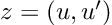
Would it be possible to teach a computer the rules of differentiation? The answer is yes! It is not only possible but can even be elegant. Enter the dual numbers! A dual number is very similar to a two-dimensional vector:

the first element represents the value of a function at a given point, and the second one is its derivative at the same point. For instance, the constant 3 will be written as the dual number (3, 0) (the 0 means that it’s a constant and thus its derivative is 0) and the variable x = 3 will be written as (3,1) (the 1 meaning that 3 is an evaluation of the variable x, and thus its derivative respective to x is 1). I know this sounds strange, but stick with me; it will become clearer later.

So, we have a new mathematical toy. We have to write down the game rules if we want to have any fun with it: let’s start defining addition, subtraction, and multiplication by a scalar. We decide they follow exactly the same rules that vectors do:

So far, nothing exciting. The multiplication is defined in a more interesting way:

Why? Because we said the second term represents a derivative, it has to follow the product rule for derivatives.

What about quotients? You guessed… the division of dual numbers follows the quotient rule for derivatives:

Last but not least, the power of a dual number to a real number is defined as:

Perhaps you feel curiosity about the multiplication by u’. This corresponds to the chain rule, and enables our dual numbers for something as desirable as function composition.

The operations defined above cover a lot of ground. Indeed, any algebraic operation can be built using them as basic components. This means that we can pass a dual number as the argument of an algebraic function, and here comes the magic, the result will be:

It is hard to overstate how powerful this is. The equation above tells us that just by feeding the function the dual number (x, 1) it will return its value at, plus its derivative! Two for the price of one!

Those readers familiar with complex numbers may find interesting to try the following exercise:

If we define a dual number as

(u, u’) = u + e u’

with e² = 0, all the properties above are automatically satisfied!

Teaching derivatives to your computer

Just as a calculus student will do, the rules of differentiation turn a calculus problem into an algebra one. And the good news: computers are better at algebra than you!

So, how can we implement these rules in a practical way on our computer? Implementing a new object (a dual number) with its own interaction rules sounds like a task for object-oriented programming. And, interestingly enough, the process is surprisingly similar to that of teaching a human student. With the difference that our “digital student” will never forget a rule, apply it the wrong way, or forget a minus sign!

So, how do these rules look, for instance, in Julia? (For a Python implementation, take a look here). First of all, we need to define a Dual object, representing a dual number. In principle, it is as simple as a container for two real numbers:

""" Structure representing a Dual number """
struct Dual
x::Real
dx::Real
end

Later, it will come in handy to add a couple of constructors.

""" Structure representing a Dual number """
struct Dual
x::Real
dx::Real

""" Default constructor """
function Dual(x::Real, dx::Real=0)::Dual
new(x, dx)
end

""" If passed a Dual, just return it
This will be handy later """
function Dual(x::Dual)::Dual
return x
end
end

Don’t worry too much if you don’t understand the lines above. They have been added only making the Dual object easier to use (for instance, Dual(1) would have failed without the first constructor, and so would have done the application of Dual to a number that is already a Dual).

Another trick that will prove handy soon is to create a type alias for anything that is either a Number (one of Julia's base types) or a Dual.

const DualNumber = Union{Dual, Number}

And now comes the fun part. We’ll teach our new object how to do mathematics! For instance, as we saw earlier, the rule for adding dual numbers is to add both their components, just as in a 2D vector:

import Base: +
function +(self::DualNumber, other::DualNumber)::Dual
self, other = Dual(self), Dual(other) # Coerce into Dual
return Dual(self.x + other.x, self.dx + other.dx)
end

We have to teach even more basic stuff. Remember a computer is dramatically devoid of common sense, so, for instance, we have to define the meaning of a plus sign in front of a Dual.

+(z::Dual) = z

This sounds as idiotic as explaining that +3 is equal to 3, but the computer needs to know! Another possibility is using inheritance, but this is an advanced topic beyond the scope of this piece.

Defining minus a Dual will also be needed:

import Base: -
-(z::Dual) = Dual(-z.x, -z.dx)

and actually, it allows us to define the subtraction of two dual numbers as a sum:

function -(self::DualNumber, other::DualNumber)::Dual
self, other = Dual(self), Dual(other) # Coerce into Dual
return self + (-other) # A subtraction disguised as a sum!
end

Some basic operations may be slightly trickier than expected. For instance, when is a dual number smaller than another dual number? Notice that in this case, it only makes sense to compare the first elements, and ignore the derivatives:

import Base: <
<(self::Dual, other::Dual) = self.x < other.x

As we saw before, more interesting stuff happens with multiplication and division:

import Base: *, /

function *(self::DualNumber, other::DualNumber)::Dual
self, other = Dual(self), Dual(other) # Coerce into Dual
y = self.x * other.x
dy = self.dx * other.x + self.x * other.dx # Rule of product for derivatives
return Dual(y, dy)
end

function /(self::DualNumber, other::DualNumber)::Dual
self, other = Dual(self), Dual(other) # Coerce into Dual
y = self.x / other.x
dy = (self.dx * other.x - self.x * other.dx) / (other.x)^2 # Rule of quotient for derivatives
return Dual(y, dy)
end

and with potentiation to a real number:

import Base: ^
function ^(self::Dual, other::Real)::Dual
self, other = Dual(self), Dual(other) # Coerce into Dual
y = self.x^other.x
dy = other.x * self.x^(other.x - 1) * self.dx # Derivative of u(x)^n
return Dual(y, dy)
end

The full list of definitions for algebraic operations is here. For Python, use this link. I recommend taking a look!

After this, each and every time our dual number finds one of the operations defined above in its mysterious journey down a function or a script, it will keep track of its effect on the derivative. It doesn’t matter how long, complicated, or poorly programmed the function is, the second coordinate of our dual number will manage it. Well, as long as the function is differentiable and we don’t hit the machine’s precision… but that would be asking our computer to do magic.

Example

As an example, let’s calculate the derivative of the polynomial:

at x = 3.

For the sake of clarity, we can compute the derivative by hand:

it is apparent that and p(3) = 39 and p’(3) = 34.

Using our Dual object, we can reach the same conclusion automatically:

poly = x -> x^3 + x^2 + x 
z = Dual(3, 1)
poly(z)

> Dual(39, 34)

Even if the same polynomial is defined in a more intricate way, the Dual object can keep track:

""" Equivalent to poly = x -> x^3 + x^2 + x
Just uglier """
function poly(x)
aux = 0 # Initialize auxiliary variable
for n in 1:3 # Add x^1, x^2 and x^3
aux = aux + x^n
end
end

poly(z)

> Dual(39, 34)

What about non-algebraic functions?

The method sketched above will fail miserably as soon as our function contains a non-algebraic element, such as a sine or an exponential. But don’t panic, we can just go to our calculus book and teach our computer some more basic derivatives. For instance, our table of derivatives tells us that the derivative of a sine is a cosine. In the language of dual numbers, this reads:

Confused about the u’? Once again, this is just the chain rule.

The rule of thumb here is, and actually was since the very beginning:

We can create a _factory function that abstracts this structure for us:

function _factory(f::Function, df::Function)::Function
return z -> Dual(f(z.x), df(z.x) * z.dx)
end

So now, we only have to open our derivatives table and fill line by line, starting with the derivative of a sine, continuing with that of a cosine, a tangent, etc.

import Base: sin, cos

sin(z::Dual) = _factory(sin, cos)(z)
cos(z::Dual) = _factory(cos, x -> -sin(x))(z) # An explicit lambda function is often required

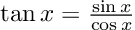
If we know our maths, we don’t even need to fill all the derivatives manually from the table. For instance, the tangent is defined as:

and we already have automatically differentiable sine, cosine, and division in our arsenal. So this line will do the trick:

import Base: tan

tan(z::Dual) = sin(z) / cos(z) # We can rely on previously defined functions!

Of course, hard-coding the tangent’s derivative is also possible, and probably good for code performance and numerical stability. But hey, it’s quite cool that this is even possible!

See a more complete derivatives table here (Python version here).

Example

Let’s compute the derivative of the non-algebraic function

It is easy to prove analytically that the derivative is 1 everywhere (notice that the argument of the tangent is actually constant). Now, using Dual:

fun = x -> x + tan(cos(x)^2 + sin(x)^2)

z = Dual(0, 1)
fun(z)

> Dual(1.557407724654902, 1.0)

Making it more user-friendly

We can use dual numbers to create a user-friendly derivative function:

"""
derivative(f)

Seamlessly turns a given function f
into
the function's derivative
"""
function derivative(f)
df = x -> f(Dual(x, 1.0)).dx
return df
end

Using this, our example above will look like:

fun = x -> x + tan(cos(x)^2 + sin(x)^2)

dfun = derivative(f)
dfun(0)

> 1.0

Another example

Now we want to calculate and visualize the derivatives of:

First, we have to input the function, and the derivative gets calculated automatically:

f(x) = x^2 - 5x + 6 - 5x^3 - 5 * exp(-50 * x^2)

df = derivative(f)

We can visualize the results by plotting a tangent line:

using Plots

I = [-0.7; 0.7]
δ = 0.025
@gif for a = [I[1]:δ:I[2]; I[2]-δ:-δ:I[1]+δ]
L(x) = f(a) + df(a) * (x - a)
plot(f, -1, 1, leg=false)
scatter!([a], [f(a)], m=(:red, 2))
plot!(L, -1, 1, c=:red)
ylims!(-5, 15)
end

Is this useful?

Automatic differentiation is particularly useful in the field of Machine Learning, where multidimensional derivatives (better known as gradients) have to be performed as fast and exactly as possible. Said this, automatic differentiation for Machine Learning is usually implemented in a different way, the so-called backward or reverse mode, for efficiency reasons.

A well-established library for automatic differentiation is JAX (for Python). Machine learning frameworks such as Tensorflow and Pytorch also implement automatic differentiation. For Julia, multiple libraries seem to be competing, but Enzyme.jl seems to be ahead. Forwarddiff.jl is also worth taking a look at.

Acknowledgments

I want to say thanks to my colleague and friend Abel Siqueira, for kindly introducing me to Julia and reviewing this post, and to Aron Jansen, for his kind and useful suggestions. A more in-depth introduction can be found in this episode of Chris Rackauckas’ book on scientific machine learning.

The TeX Math Here browser add-in also played an important role: it allowed me to transfer my Latex equations from Markdown to Medium in an (almost) painless way.


Automatic differentiation from scratch was originally published in Netherlands eScience Center on Medium, where people are continuing the conversation by highlighting and responding to this story.