Atomic Orbitals

Prerequiresites: Quantum Mechanics course

Electrons around a nucleus. Do they look like little well behaved planets orbiting a sun?

NOPE!

We get spread out blobs in special little patterns called orbitals. Here, we will look at their shapes and properties a bit. Today we will look at graphs in 1D and 2D, but the next post, Atomic Orbitals Pt. 2, uses a fancy, but slightly unstable plotting package, GLVisualize to generate some 3D plots.

The Hamiltonian for our problem is:

begin{equation}
{cal H}Psi(mathbf{x}) =left[ -frac{hbar}{2 m} nabla^2 – frac{Z e^2}{4 pi epsilon_0 r}right]Psi(mathbf{x}) = E Psi(mathbf{x})
end{equation}
with
begin{equation}
nabla^2= frac{1}{r^2}frac{partial}{partial r} left(
r^2 frac{partial}{partial r}
right)+
frac{1}{r^2 sin theta} frac{partial}{partial theta} left(
sin theta frac{partial}{partial theta}
right)+
frac{1}{r^2 sin^2 theta} frac{partial^2}{partial phi^2}
end{equation}

To solve this problem, we begin by guessing a solution with separated radial and angular variables,
begin{equation}
Psi(mathbf{x}) = R(r) Theta ( theta,phi)
end{equation}

begin{equation}
frac{E r^2 R(r)}{2r R^{prime}(r) + r^2 R^{prime prime}(r)}=
frac{left( frac{1}{sin theta} frac{partial}{partial theta} left(
sin theta frac{partial Theta(theta,phi)}{partial theta}
right)+
frac{1}{sin^2 theta} frac{partial^2 Theta(theta,phi)}{partial phi^2}right) }{Theta( theta, phi)}
=C
end{equation}

Instead of going into the precise mechanisms of solving those two separate equations here, trust for now that they follow standard special functions, the associated Legendre polynomial and the generalized Laguerre polynomial. Try a standard quantum mechanics textbook for more information about this.

begin{equation}
Y^m_l(θ,ϕ) = (-1)^m e^{i m phi} P^m_l (cos(θ))
end{equation}
where $P^m_l (cos (theta))$ is the associated Legendre polynomial.

begin{equation}
R^{n,l} ( rho ) = rho ^l e^{- rho /2} L^{2 l+1}_{n-l-1} ( rho )
end{equation}
where $L^{2 l+1}_{n-l-1}(rho)$ is the generalized Laguerre polynomial.

begin{equation}
rho=frac{2r}{n a_0}
end{equation}

begin{equation}
N=sqrt{left(frac{2}{n}right)^3 frac{(n-l-1)}{2n(n+l)!}}
end{equation}

#Pkg.update();
#Pkg.add("GSL");
#Pkg.add("PyPlot");
using GSL;    #GSL holds the special functions
using PyPlot;

Cell to Evaluate

What’s below is a bunch of definitions that makes our calculations easier later on. Here I utilize the GNU scientific library, GSL imported above, to calculate the special functions.

Programming Tip!

Even though it’s not necessary, specifying the type of inputs to a function through m::Int helps prevent improper inputs and allows the compiler to perform additional optimizations. Julia also implements abstract types, so we don’t have to specify the exact type of Int. Real allows a numerical, non-complex type.

Type Greek characters in Jupyter notebooks via LaTeX syntax, e.g. alpha+tab

The function Orbital throws DomainError() when l or m do not obey their bounds. Julia supports a wide variety of easy to use error messages.

a0=1; #for convenience, or 5.2917721092(17)×10−11 m

# The unitless radial coordinate
ρ(r,n)=2r/(n*a0);

#The θ dependence
function Pmlh(m::Int,l::Int,θ::Real)
    return (-1.0)^m *sf_legendre_Plm(l,m,cos(θ));
end

#The θ and ϕ dependence
function Yml(m::Int,l::Int,θ::Real,ϕ::Real)
    return  (-1.0)^m*sf_legendre_Plm(l,m,cos(θ))*e^(im*m*ϕ)
end

#The Radial dependence
function R(n::Int,l::Int,ρ::Real)
    if isapprox(ρ,0)
        ρ=.01
    end
     return sf_laguerre_n(n-l-1,2*l+1,ρ)*e^(-ρ/2)*ρ^l
end

#A normalization: This is dependent on the choice of polynomial representation
function norm(n::Int,l::Int)
    return sqrt((2/n)^3 * factorial(n-l-1)/(2n*factorial(n+l)))
end

#Generates an Orbital function of (r,θ,ϕ) for a specified n,l,m.
function Orbital(n::Int,l::Int,m::Int)
    if l>n    # we make sure l and m are within proper bounds
        throw(DomainError())
    end
    if abs(m)>l
        throw(DomainError())
    end
    psi(ρ,θ,ϕ)=norm(n, l)*R(n,l,ρ)*Yml(m,l,θ,ϕ);
    return psi
end

#We will calculate is spherical coordinates, but plot in Cartesian, so we need this array conversion
function SphtoCart(r::Array,θ::Array,ϕ::Array)
    x=r.*sin(θ).*cos(ϕ);
    y=r.*sin(θ).*sin(ϕ);
    z=r.*cos(θ);
    return x,y,z;
end

function CarttoSph(x::Array,y::Array,z::Array)
    r=sqrt(x.^2+y.^2+z.^2);
    θ=acos(z./r);
    ϕ=atan(y./x);
    return r,θ,ϕ;
end

"Defined Helper Functions"

Parameters

Grid parameters:
You might need to change rmax to be able to view higher $n$ orbitals.

Remember that
begin{equation}
0<n ;;;;; ;;;; 0 leq l < n ;;;;; ;;;; -l leq m leq l
;;;;; ;;;; n,l,m in {cal Z}
end{equation}

# Grid Parameters
rmin=.05
rmax=10
Nr=100 #Sampling frequency
Nθ=100
Nϕ=100

# Choose which Orbital to look at
n=3;
l=1;
m=0;
"Defined parameters"
#Linear Array of spherical coordinates
r=collect(linspace(rmin,rmax,Nr));
ϕ=collect(linspace(0,2π,Nθ));
θ=collect(linspace(0,π,Nϕ));
#3D arrays of spherical coordinates, in order r,θ,ϕ
ra=repeat(r,outer=[1,Nθ,Nϕ]);
θa=repeat(transpose(θ),outer=[Nr,1,Nϕ]);
ϕa=repeat(reshape(ϕ,1,1,Nϕ),outer=[Nr,Nθ,1]);

x,y,z=SphtoCart(ra,θa,ϕa);

Though I could create a wrapped up function with Orbital(n,l,m) and evaluate that at each point, the below evaluation takes advantage of the separability of the solution with respect to spherical dimensions. The special functions, especially for higher modes, take time to calculate, and the fewer calls to GSL, the faster the code will run. Therefore, this implementation copies over radial and angular responses.

Ψ=zeros(Float64,Nr,Nϕ,Nθ)
θd=Int64(round(Nθ/2))  ## gives approximately the equator.  Will be useful later

p1=Pmlh(m,l,θ[1]);
p2=exp(im*m*ϕ[1]);
for i in 1:Nr
    Ψ[i,1,1]=norm(n,l)*R(n,l,ρ(r[i],n))*p1*p2;
end

for j in 1:Nθ
    Ψ[:,j,1]=Ψ[:,1,1]*Pmlh(m,l,θ[j])/p1;
end

for k in 1:Nϕ
    Ψ[:,:,k]=Ψ[:,:,1]*exp(im*m*ϕ[k])/p2;
end
pygui(false)
xlabel("θ")
ylabel("Ψ")
title("Wavefunction for n= $n ,l= $l ,m= $m ")

annotate("l= $l Angular Node",
xy=[π/2;0],
xytext=[π/2+.1;.02],
xycoords="data",
arrowprops=Dict("facecolor"=>"black"))

plot(θ,zeros(θ))
plot(θ,reshape(Ψ[50,:,1],100)) #reshape makes Ψ 1D

2p Angle Slice

A slice along the θ plane showing an angular node for the 2p orbital.

pygui(false)
xlabel("r")
ylabel("Ψ")
title("Wavefunction for n= $n ,l= $l ,m= $m ")

plot(r,zeros(r))
plot(r,reshape(Ψ[:,50,1],100)) #reshape makes Ψ 1D

3p Radial Slice

A slice along the radial plane showing a radial node in the 3p orbital.

#rap=squeeze(ra[:,:,50],3)
#θap=squeeze(θa[:,:,50],3)
#ϕap=squeeze(ϕa[:,:,50],3)
#Ψp=squeeze(Ψ[:,:,50],3)
rap=ra[:,:,50]
θap=θa[:,:,50]
ϕap=ϕa[:,:,50]
Ψp=Ψ[:,:,50]
xp,yp,zp=SphtoCart(rap,θap,ϕap);
pygui(false)
xlabel("x")
ylabel("z")
title("ϕ-slice of Ψ for n=$n, l=$l, m=$m")
pcolor(xp[:,:],zp[:,:],Ψp[:,:],cmap="coolwarm")
colorbar()

3p in 2d

Slice of a 3p orbital in the x and z plane.
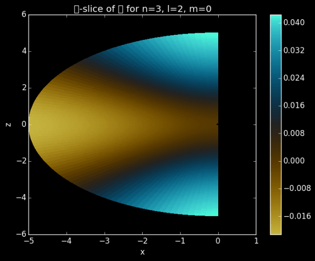
3dz2 in 2d

Slice of a 3dz2 orbital in the x and z plane.

Don’t forget to check out Atomic Orbitals Pt. 2!

Atomic Orbitals Pt. 2

Prerequiresites: Quantum Mechanics course

If you haven’t read it already, check out Atomic Orbitals Pt. 1. Today, we try and make some prettier pictures. GLVisualize is quite a beautiful package, but not entirely the easiest to use at this point with some not so consistent documentation.

To add this package:

Pkg.add("GLVisualize")

and test with:

Pkg.test("GLVisualize")

But, other steps may be necessary to get the package working. On a Mac, I was required to install the Homebrew.jl package.

#Pkg.update();
#Pkg.add("GSL");
using GSL;
using GLVisualize;
a0=1; #for convenience, or 5.2917721092(17)×10−11 m

# The unitless radial coordinate
ρ(r,n)=2r/(n*a0);

#The θ dependence
function Pmlh(m::Int,l::Int,θ::Real)
    return (-1.0)^m *sf_legendre_Plm(l,m,cos(θ));
end

#The θ and ϕ dependence
function Yml(m::Int,l::Int,θ::Real,ϕ::Real)
    return  (-1.0)^m*sf_legendre_Plm(l,abs(m),cos(θ))*e^(im*m*ϕ)
end

#The Radial dependence
function R(n::Int,l::Int,ρ::Real)
    if isapprox(ρ,0)
        ρ=.001
    end
     return sf_laguerre_n(n-l-1,2*l+1,ρ)*e^(-ρ/2)*ρ^l
end

#A normalization: This is dependent on the choice of polynomial representation
function norm(n::Int,l::Int)
    return sqrt((2/n)^3 * factorial(n-l-1)/(2n*factorial(n+l)))
end

#Generates an Orbital Funtion of (r,θ,ϕ) for a specificied n,l,m.
function Orbital(n::Int,l::Int,m::Int)
    if (l>n)    # we make sure l and m are within proper bounds
        throw(DomainError())
    end
    if abs(m)>l
       throw(DomainError())
    end
    psi(ρ,θ,ϕ)=norm(n, l)*R(n,l,ρ)*Yml(m,l,θ,ϕ);
    return psi
end

#We will calculate is spherical coordinates, but plot in cartesian, so we need this array conversion
function SphtoCart(r::Array,θ::Array,ϕ::Array)
    x=r.*sin(θ).*cos(ϕ);
    y=r.*sin(θ).*sin(ϕ);
    z=r.*cos(θ);
    return x,y,z;
end

function CarttoSph(x::Array,y::Array,z::Array)
    r=sqrt(x.^2+y.^2+z.^2);
    θ=acos(z./r);
    ϕ=atan(y./x);
    return r,θ,ϕ;
end

"Defined Helper Functions"

Here, create a square cube, and convert those positions over to spherical coordinates.

range=-10:.5:10
x=collect(range);
y=collect(range);
z=collect(range);
N=length(x);
xa=repeat(x,outer=[1,N,N]);
ya=repeat(transpose(y),outer=[N,1,N]);
za=repeat(reshape(z,1,1,N),outer=[N,N,1]);
println("created x,y,z")

r,θ, ϕ=CarttoSph(xa,ya,za);
println("created r,θ,ϕ")
Ψ=Orbital(3,2,-1)
Ψp=Orbital(3,1,0)
Ψv = zeros(Float32,N,N,N);
ϕv = zeros(Float32,N,N,N);
for nn in 1:N
    for jj in 1:N
        for kk in 1:N
            val=Ψ(ρ(r[nn,jj,kk],2),θ[nn,jj,kk],ϕ[nn,jj,kk]);
            #val+=Ψp(ρ(r[nn,jj,kk],2),θ[nn,jj,kk],ϕ[nn,jj,kk]);
            Ψv[nn,jj,kk]=convert(Float32,abs(val));
            ϕv[nn,jj,kk]=convert(Float32,angle(val));
        end
    end
end

mid=round(Int,(N-1)/2+1);
Ψv[mid,mid,:]=Ψv[mid+1,mid+1,:]; # the one at the center diverges
Ψv=(Ψv-minimum(Ψv))/(maximum(Ψv)-minimum(Ψv) );
w,r = glscreen()

robj=visualize(Ψv)

#choose this one for surfaces of constant of intensity
view(visualize(robj[:intensities],:iso))

#choose this for a block of 3D density
#view(visualize(Ψv))
r()

2p Orbital

2p

2p Orbital block showing the density of the wavefunction.

2p

2p Orbital shown via isosurface.

3d orbitals

3d0

3dz2 Orbital shown via isosurface. This corresponds to $n=3$, $l=2$, $m=0$.

3dm1

A 3d Orbital shown via isosurface. This corresponds to $n=3$, $l=2$, $m=-1$. This is not one of the canonical images, but instead an $m$ shape.

3dxy

3dxy (x2-y2) orbital shown in density. This is the sum of an $m=-2$ and $m=2$ state, for $n=3,l=2$.

3p

In order to get this 3p surface image to come out correctly, I used the square root of the values instead in order to be able to see the much fainter outer lobe.

3p

3p surface plot.

3p

3p space plot.

Jacobi Transformation of a Symmetric Matrix

Based on Numerical Recipes in C++, Sec 11.1

So you want to diagonalize a matrix, do you?
Well, if you have a tiny symmetric matrix, you REALLY want to write up the algorithm by hand, and don’t want to spend much time trying to understand the algorithm, then you have come to the right place.

Otherwise, use LAPACK/BLAS to call a highly optimized routine that can work extremely quickly on large matrices. Julia has those libraries built in already. Even if you do call those matrices, you can make them work better by understanding what’s going on underneath the hood, which is why we are going through this now.

Start with a base rotation matrix of the Form

From our starting arbitrary symmetric ,

we will run a series of transformations,

where each iteration brings closer to diagonal form. Thus in our implementing our algorithm, we need to determine two things

  • The values of and
  • The pattern of sweeping and

And in the end we will need to finally determine if this actually converges, and if has any sort of efficiency.

So lets expand one transformation, and we if we can solve for $c$ and $s$.

Determining $s$ and $c$

Given we specifically want $a^{prime}_{pq}$ to be zero, we re-arrange the last equation,

At first glance, this equation might not look easier to solve for $s$ or $c$. At second glance either. We define a new parameter $t = s/c$, which now makes the equation,

now quite easily solvable by our friendly quadratic formula. Though the book does recommend using a form that pulls out smaller roots through

Then reverse solve back to

Though we could use the expressions above, if we simplify them with our new expressions for $c$ and $s$ analytically, we reduce computational load and round off error. These new expressions are

with the new variable

Convergence

The sum of the squares of the off diagonal elements, choosen in either upper or lower triangles arbitrarily,

Eigenvectors

By forming a product of every rotation matrix, we also come to approximate the matrix $V$ where

and $D$ is the diagonal form of $A$. $V$ is computed through iterative computation

Enough with the talking! LETS COMPUTE STUFF

# First, Lets make our nice, helpful functions

## A function to look at the convergence
function convergence(A::Array)
    num=0.0
    l=size(A)[1]
    for ii in 1:(l-1)
        for jj in (ii+1):l ## just looking at the lower triangle
            num+=A[ii,jj]^2
            #println(ii,' ',jj,' ',num,' ',A[ii,jj])
        end
    end
    return num
end

This makes a matrix easier to look at than when its filled
with 1.043848974e-12 everywhere

function roundmatrix(A::Array,rtol::Real)
    Ap=copy(A)
    for ii in 1:length(A)
        if abs(Ap[ii])<rtol
            Ap[ii]=0
        end
    end
    return Ap;
end
## Here we create a random symmetric matrix
function makeA(n::Int)
    A=randn(n,n);
    for ii in 1:n
        A[ii,1:ii]=transpose(A[1:ii,ii])
    end
    V=eye(n) #initializing the orthogonal transformation
    return A,copy(A),V
end
## One A returned will be stored to compare initial and final

Now on to the rotations!

We don’t always want to compute the eigenvectors, so those are in the optional entries slot.
Both tell the function to compute the vectors with computeV=true
and input the V=V after the semicolon.

function Rotate(A::Array,p::Int,q::Int; computeV=false, V::Array=eye(1))
    θ=(A[q,q]-A[p,p])/(2*A[p,q]);
    t=sign(θ)/(abs(θ)+sqrt(θ^2+1));

    c=1/sqrt(t^2+1)
    s=t*c
    τ=s/(1+c)

    l=size(A)[1]
    Ap=copy(A[:,p])
    Aq=copy(A[:,q])
    for r in 1:l
        A[r,p]=Ap[r]-s*(Aq[r]+τ*Ap[r])
        A[r,q]=Aq[r]+s*(Ap[r]-τ*Aq[r])

        A[p,r]=A[r,p]
        A[q,r]=A[r,q]
    end
    A[p,q]=0
    A[q,p]=0
    A[p,p]=Ap[p]-t*Aq[p]
    A[q,q]=Aq[q]+t*Aq[p]

    if computeV==true
        Vp=copy(V[:,p])
        Vq=copy(V[:,q])
        for r in 1:l
            V[r,p]=c*Vp[r]-s*Vq[r]
            V[r,q]=s*Vp[r]+c*Vq[r]
        end
        return A,V
    else
        return A;
    end
end

This function performs one sweep


function Sweep(A;compV=false,V=eye(1))
    n=size(A)[1]
    for ii in 2:n
        for jj in 1:(ii-1) ## Just over one triangle
            if compV==false
                A=Rotate(A,ii,jj)
            else
                A,V=Rotate(A,ii,jj;computeV=true,V=V);
            end
        end
    end

    if compV==false
        return A
    else
        return A,V
    end
end

Just creating some size of matrix

A,A0,V=makeA(5);
## keep evaluating for a couple iterations
## watch how it changes
A,V=Sweep(A;compV=true,V=V);
roundmatrix(A,1e-10),A,V,convergence(A)

This output is after several sweeps

    (
    5x5 Array{Float64,2}:
     -1.59942  0.0       0.0       0.0      0.0
      0.0      1.03678   0.0       0.0      0.0
      0.0      0.0      -0.823094  0.0      0.0
      0.0      0.0       0.0       3.09433  0.0
      0.0      0.0       0.0       0.0      1.3409,

    5x5 Array{Float64,2}:
     -1.59942      5.1314e-30    2.32594e-36  -9.54088e-49  -1.22782e-53
      5.1314e-30   1.03678       2.65014e-38   9.13791e-56   6.64996e-67
      2.32594e-36  2.65014e-38  -0.823094     -9.56652e-61   2.08002e-92
     -9.54088e-49  9.13791e-56  -9.56652e-61   3.09433       0.0
     -1.22782e-53  6.64996e-67   2.08002e-92   0.0           1.3409     ,

    5x5 Array{Float64,2}:
      0.0537334   0.0599494  -0.735228  0.139      0.658511
      0.310018    0.612957   -0.14049   0.611348  -0.367001
      0.759653   -0.475834    0.264118  0.282571   0.216575
     -0.480405   -0.546544   -0.132383  0.644217  -0.194831
     -0.305189    0.30913     0.593648  0.33477    0.588905,

    2.6331310238375346e-59)

Compare the Optimized LAPLACK routine to your results

eig(A0)
      ([-1.599424470672961,-0.8230937166650976,1.0367806031602211,
      1.3408963512476402,3.0943321944116593],
      5x5 Array{Float64,2}:
       -0.0537334   0.735228   0.0599494  -0.658511  -0.139
       -0.310018    0.14049    0.612957    0.367001  -0.611348
       -0.759653   -0.264118  -0.475834   -0.216575  -0.282571
        0.480405    0.132383  -0.546544    0.194831  -0.644217
        0.305189   -0.593648   0.30913    -0.588905  -0.33477 )
## A good check to make sure V is an orthonomal transformation
roundmatrix(V*A*transpose(V)-A0,1e-12)
      5x5 Array{Float64,2}:
       0.0  0.0  0.0  0.0  0.0
       0.0  0.0  0.0  0.0  0.0
       0.0  0.0  0.0  0.0  0.0
       0.0  0.0  0.0  0.0  0.0
       0.0  0.0  0.0  0.0  0.0

How long does it take to make a Sweep?
How much memory will the computation take?
This is dependent on how large the matrix is, and determines whether or not we
want to use this algorithm.


A,A0,V=makeA(10);
@time Sweep(A);
A,A0,V=makeA(20);
@time Sweep(A);
A,A0,V=makeA(100);
@time Sweep(A);
  0.000028 seconds (320 allocations: 30.469 KB)
  0.000099 seconds (1.33 k allocations: 187.266 KB)
  0.007413 seconds (34.66 k allocations: 17.448 MB, 14.20% gc time)

In addition to time per sweep, we need to know how many sweeps we need to run. So again we run it on a 10×10, 20×20, and 100×100. The efficiency of the algorithm would get a lot worse if we have to sweep the 100×100 a bunch of times.

A10,Ap10,V=makeA(10);
A20,Ap20,V=makeA(20);
A100,Ap100,V=makeA(100);
nsweep=collect(1:7);
conv10=zeros(7)
conv20=zeros(7)
conv100=zeros(7)
for i in nsweep
    A10=Sweep(A10)
    A20=Sweep(A20)
    A100=Sweep(A100)
    conv10[i]=convergence(A10)
    conv20[i]=convergence(A20)
    conv100[i]=convergence(A100)
end

[nsweep conv10/10 conv20/20 conv100/100]
7x4 Array{Float64,2}:
 1.0  1.10944       2.43759      14.6644
 2.0  0.105628      0.312076      2.87182
 3.0  0.000265288   0.017073      0.498082
 4.0  6.64324e-9    0.000119472   0.0390564
 5.0  4.05463e-18   3.56679e-11   0.00133833
 6.0  3.17274e-42   1.96318e-23   6.07661e-7
 7.0  6.76289e-110  4.07871e-49   3.98102e-13

Well, so we’ve seen how to do one form of exact diagonalization that works, but doesn’t scale very well up to 100×100 matrices. So stay tuned for the Householder method, hopefully coming up soon.

Until then, happy computing 🙂