Julia – The Artificial Intelligence Computer Programming Language for the Next 150 Years

Hollywood, CA – Do you know what programming language will be used for artificial intelligence in the Year 2150?

According to TV science fiction drama The 100, the answer is Julia.

The 100 tells the story of a post-apocalyptic Earth shaped by artificial intelligence.

In Season 3, Episode 12, Raven Reyes, performed by Lindsey Morgan, discovers code that enables her team to access A.L.I.E. 2.0, the latest version of the most important artificial intelligence program in the world.

A screenshot reveals that the crucial code is written in Julia and copied from the Julia language repository on GitHub.

According to Viral Shah, co-creator of the Julia language and CEO of Julia Computing, “The 100 staff did their research. It makes sense that they would use Julia to represent the language of artificial intelligence in 2150. Today Julia is being used to guide self-driving race cars and diagnose serious medical conditions. Julia is the most expressive and most powerful language for artificial intelligence today, and based on current growth, this trend will continue to accelerate in the months and years ahead.”


Screenshot from The 100 and the Julia language GitHub repository
from which it was copied

The 100 is not the only Hollywood television program featuring Julia.

Julia also made an appearance on Casual, season 3, episode 5. During this episode, the lead character, Alex, interviews for a Chief Technology Officer position at a technology startup company. “The people we meet your age,” the interviewer says to Alex, “they’re not versed in the newer languages: Swift, Julia, Google Go.”

Shah explained, “The character interviewing Alex in Casual hasn’t had quite enough experience with Julia programmers. While it’s true that Julia adoption has exploded among young people – especially at universities and at fast-growing companies including Amazon, Apple, Facebook, Google and Uber – data scientists and researchers with decades of experience are also flocking to Julia to take advantage of Julia’s superior performance and easy-to-learn syntax. Examples include Nobel Laureate Thomas J. Sargent who describes himself as a “walking advertisement for Julia,” and the engineering manager at a major US industrial firm who wrote to tell us:

“I just wanted to thank you for Julia. I am the manager of an engineering group responsible for quite a few numerical tools from stand-alone small programs to full-blown finite element codes. Julia is the most exciting thing I’ve seen in years. When a language is cool enough for a 50-something year old manager to spend his spare time programming in it at home, you know that you’ve kindled serious excitement.”

About Julia and Julia Computing

Julia is the fastest modern high performance open source computing language for data, analytics, algorithmic trading, machine learning and artificial intelligence. Julia combines the functionality and ease of use of Python, R, Matlab, SAS and Stata with the speed of C++ and Java. Julia delivers dramatic improvements in simplicity, speed, capacity and productivity. Julia provides parallel computing capabilities out of the box and unlimited scalability with minimal effort. With more than 1 million downloads and +161% annual growth, Julia is one of the top 10 programming languages developed on GitHub and adoption is growing rapidly in finance, insurance, energy, robotics, genomics, aerospace and many other fields.

Julia users, partners and employers hiring Julia programmers in 2017 include Amazon, Apple, BlackRock, Capital One, Comcast, Disney, Facebook, Ford, Google, Grindr, IBM, Intel, KPMG, Microsoft, NASA, Oracle, PwC, Raytheon and Uber.

  1. Julia is lightning fast. Julia provides speed improvements up to
    1,000x for insurance model estimation, 225x for parallel
    supercomputing image analysis and 11x for macroeconomic modeling.

  2. Julia is easy to learn. Julia’s flexible syntax is familiar and
    comfortable for users of Python, R and Matlab.

  3. Julia provides unlimited scalability. Julia applications can be deployed on large clusters with a click of a button and can run parallel and distributed computing quickly and easily on tens of thousands of nodes.

  4. Julia integrates well with existing code and platforms. Users of
    Python, R, Matlab and other languages can easily integrate their
    existing code into Julia.

  5. Elegant code. Julia was built from the ground up for
    mathematical, scientific and statistical computing, and has advanced
    libraries that make coding simple and fast, and dramatically reduce
    the number of lines of code required – in some cases, by 90%
    or more.

  6. Julia solves the two language problem. Because Julia combines
    the ease of use and familiar syntax of Python, R and Matlab with the
    speed of C, C++ or Java, programmers no longer need to estimate
    models in one language and reproduce them in a faster
    production language. This saves time and reduces error and cost.

Julia Computing was founded in 2015 by the creators of the open source Julia language to develop products and provide support for businesses and researchers who use Julia.
Automatic differentiation of discontinuous integrals

By: Tamás K. Papp

Re-posted from: https://tamaspapp.eu/post/discontinuous_integral_ad/

This is a much simplified writeup of a problem I encountered, in a self-contained blog post.

You want to approximate the integral

\[
I(\theta) = \int 1(g(x) > 0) f(x,\theta) dx
\]

where \(g\) is a continuous function, and \(f(x,\theta)\) is a parametric distribution over \(x\). Everthing is continous, and thus \(I\) is, too.

You face the following constraints:

  1. \(g\) is a black box. We will pretend that you can’t invert it (except for checking our results, of course).

  2. You can calculate the probability density function \(f\) and even draw \(x\)‘s for a particular \(\theta\), but that’s pretty much it. You don’t even get a cdf! (Again, except for checking our results.)

Using Monte Carlo methods, you can do the following:

  1. draw \(x_i \sim F(\cdot, \theta)\), \(i=1,\dots,N\),

  2. approximate

\[
I(\theta) \approx \frac{1}{N}\sum_i 1(g(x_i) > 0)
\]

You could code this in Julia as

d = distr(θ)   # suppose this returns some distribution that supports Base.rand
x = rand(d, N)
mean(g.(x) > 0)

So far, neat and simple. Now, the fly in the ointment: you need the derivative \(I'(\theta)\) for optimization or Hamiltonian Monte Carlo. The problem is that you cannot ForwardDiff your way through the code above: AD’ing a discontinuous step function will just give you \(0\), and rand does not work with ForwardDiff.Duals anyway (which is very sensible).

However, there is a solution: rewrite the approximation as

\[
I(\theta; \theta_0) \approx \frac{1}{N}\sum_i 1(g(x_i) > 0) \frac{f(x_i,\theta)}{f(x_i,\theta_0)}
\]

where \(\theta_0\) is the parameter used to simulate the \(x_i\). Differentiate the above at \(\theta = \theta_0\). This approximates

\[
I'(\theta) = \int 1(g(x) > 0) \frac{\partial f(x,\theta)/\partial \theta}{f(x,\theta)}f(x,\theta) dx = \int 1(g(x) > 0) \partial f(x,\theta)/\partial \theta dx
\]

which is exactly what you want.

Assume that the actual calculation is very complicated, so we would rather avoid implementing it for the integral and the derivative separately. It turns out that this is very simple to do with ForwardDiff.Dual values: the code is literally a one-liner and a fallback method:

elasticity(x::Real) = one(x)
elasticity(x::Dual{T,V,N}) where {T,V,N} = Dual{T}(one(V), partials(x) / value(x))

which you can use in a function like

integral_approx(g, d, x) = mean((g.(x) .> 0) .* elasticity.(pdf.(d, x)))

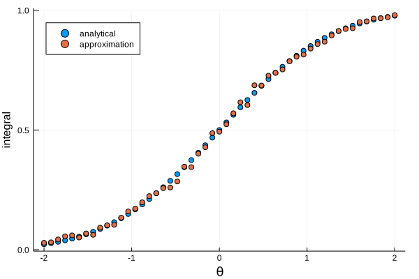
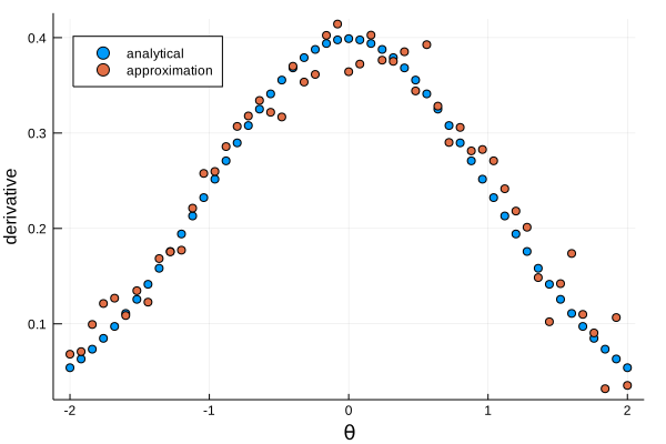
I demonstrate this with \(g(x) = x\) and \(x \sim \text{Normal}(\theta, 1)\), for which of course we know that the analytical values for \(I\) and \(I’\) are the right tail probability and the pdf at 0, respectively.

Graphs below show that the approximation is reasonable — we could make it much better with low-discrepancy sequences, but that is an orthogonal issue.

integral

derivative

It is amazing how much you can accomplish with two lines of code in Julia! The problem that motivated this blog post is multivariate with irregular regions over which \(\{ x: g(x) > 0 \}\), but I used elasticity as above.

Self-contained code for everything is available below.

download as code.jl

using ForwardDiff
import ForwardDiff: Dual, value, partials, Tag
using Distributions
using Plots
using LaTeXStrings
gr()

######################################################################
# elasticity calculation
######################################################################

"""
    elasticity(x)

Calculate `x/x`, stripping `x` of partial derivative information. Useful for
calculating elasticities of the form `∂f/f` using ForwardDiff.
"""
elasticity(x::Real) = one(x)

elasticity(x::Dual{T,V,N}) where {T,V,N} = Dual{T}(one(V), partials(x) / value(x))

######################################################################
# example application
######################################################################

integral_approx(g, d, x) = mean((g.(x) .> 0) .* elasticity.(pdf.(d, x)))

"Helper function that returns the value and derivative at the same time."
function value_and_derivative(f::F, x::R) where {F,R<:Real}
    T = typeof(Tag(F, R))
    y = f(Dual{T}(x, one(x)))
    value(y), partials(y, 1)
end

distr(θ) = Normal(θ, 1)

g(x) = x

function ID_analytical(θ)
    d = distr(θ)
    ccdf(d, 0), pdf(d, 0)
end

function ID_approx(θ)
    x = rand(distr(θ), 1000)
    value_and_derivative(θ->integral_approx(g, distr(θ), x), θ)
end

θs = linspace(-2, 2, 51)
ID0s = ID_analytical.(θs)
ID1s = ID_approx.(θs)

scatter(θs, first.(ID0s), xlab = "\\theta", ylab = "integral",
        label = "analytical", legend = :topleft)
scatter!(θs, first.(ID1s), label = "approximation")
savefig("integral.svg")

scatter(θs, last.(ID0s), xlab = "\\theta", ylab = "derivative",
        label = "analytical", legend = :topleft)
scatter!(θs, last.(ID1s), label = "approximation")
savefig("derivative.svg")