Machine-learned preconditioners – Part 1

By: Random blog posts about machine learning in Julia

Re-posted from: https://rkube.github.io/jekyll/update/2021/03/02/neural-networks-and-iterative-solvers.html

What is a preconditioner?

A common task in scientific computing is to solve a system of linear equations

\[Ax = b\]

with a matrix \(A \in \mathcal{R}^{d \times d}\) that gives the coefficients of the
system, a right-hand-side vector \(b \in \mathcal{R}^{d}\),
and a solution vector \(x \in \mathcal{R}^{d}\).

Instead of solving the linear problem directly, one often solves
the preconditioned problem. We write this problem by inserting a one in the
linear system and re-parenthesing:

\(\left( A P^{-1} \right) \left( P x \right) = b\)
In this equation we have changed the coefficient matrix from \(A\) to
\(A P^{-1}\) and the solution vector is now \(P x\) instead of \(x\). To
retrieve the original vector, simply calculate \(x = P^{-1}y\). The matrix
\(P^{-1}\) is called the preconditioner.

The dependence of \(P^{-1}\) on \(x\) is by choice. There is no deeper reason
for why the preconditioner should depend on the initial guess for the iteraion.
We choose to include this dependency here to foreshadow later applications, where
such a dependency may be useful. In practice, this choice here is rather limiting.
Since the matrix \(A_0 P^{-1}\) needs to be positive definite, and by construction
only \(\widetilde{b}\) is positive definite, the method as constructed here is only
valid for \(x \approx 0\).

The Gauss-Seidel method is an iterative method to find the solution of
a linear system. Given an initial guess \(x_0\), update the entries of this
vector following an iterative scheme and after some, or many, iterations, \(x_0\)
solves the equation \(A x_0 = b\).
Wikipedia has a nice
and instructive page on this scheme.

A good preconditioner gives you a converged solution after fewer iterations.
In other words, with a good preconditioner you are closer to the true solution
of the linear system after N iterations than you are with a bad preconditioner.
Choosing a good preconditioner depends on the problem at hand and can become
a dark art. Let’s make it even more dark and train a neural network to be
a preconditioner.

Modeling preconditioner as a neural network

As a first step, let’s model \(P^{-1}\) as a multi-layer perceptron
(technically a single-layer):

\[P^{-1} = \sigma \left( W x + \widetilde{b} \right)\]

with a weight matrix \(W \in \mathcal{R}^{d^2 \times d}\), a bias
\(\widetilde{b} \in \mathcal{R}^{d^2}\), and a ReLU \(\sigma\). With
\(x \in \mathcal{R}^{d}\) the matrix dimensions are chosen such that \(P^{-1}\)
is of dimension \(d^2\). Simply reshape it to \(d \times d\) to have it act like
a matrix.

Here I’m discussing a simple test case and am working with the Gauss-Seidel
iterative solver. For real problem one would probably use a different iterative
algorithm, but it serves as a proof-of-concept. Anyway, for Gauss-Seidel to work,
the system coefficient matrix \(AP^{-1}\) needs to be positive-definite.
How do we do this for our neural network? A simple hack is to consider only
vectors whose entries are close to zero.

That way we get away with requiring only \(\widetilde{b}\) to be
positive-definite. We get the last property by letting
\(\widetilde{b} = b_0 b_0^{T}\) and sampling the entries of \(b_0\) as
\(b_{ij} \sim \mathcal{N}(0, 1)\). In a similar fashion, we sample the entries
of the weight-matrix \(W\) as \(w_{i,j} \sim \mathcal{N}(0,1)\).

How can we train a preconditioner

To make this preconditioner useful, the weights \(W\) and bias term \(b\) need
to be optimized such that the residual after \(N\) iterations is as small
as possible. And this needs to be true for all vectors from a training set.
Using automatic differentiation, we can train \(W\) and \(b\) using gradient
descent like this:

  • Pick an initial guess \(x_0\) with \(x_{0,i} \sim \mathcal{N}(0, 0.01)\)
  • Build the preconditioner \(P^{-1} = \sigma(W, x_0, \widetilde{b})\)
  • Calculate 5 Gauss-Seidel steps. Let’s call the solution here \(y_5\).
  • Un-apply the preconditioner: \(x_5 = P^{-1} y_5\)
  • Calculate the distance to the true solution \(\mathcal{L} = \frac{1}{N} \sum_{i=1}^{N} \left( x_{\text{true}, i} – x_{5,i} \right)^2\)
  • Calculate the gradients \(\nabla_{W} \mathcal{L}\) and
    \(\nabla_{B} \mathcal{L}\)
  • Update the weight matrix and bias using gradient descent: \(W \leftarrow W – \alpha \nabla_{W} \mathcal{L}\) and \(b \leftarrow b – \alpha \nabla_{b} \mathcal{L}\). Here \(\alpha\) is the learning rate

The approach here is to directly back-propagate from the loss function \(\mathcal{L}\), through
the numerical solver, to the parameters of the preconditioner \(W\) and \(b\).
We are not working with an offline training and test-data set, but the data is
taken directly from the numerical calculations. This way we directly capture the
reaction of the numerical solver to updates proposed by gradient descent.

The derivatives \(\nabla_\theta \mathcal{L}\) can be calculate using automatic differentiation
packges, such as Zygote.

Implementation


# Test differentiation through control flow

# Use a iterative conjugate solver with preconditioner

using Random
using Zygote
using LinearAlgebra
using Distributions
using NNlib

I copy-and-pasted the Gauss-Seidel code from wikipedia:

function gauss_seidel(A, b, x, niter)
    # This is from https://en.wikipedia.org/wiki/Gauss%E2%80%93Seidel_method
    x_int = Zygote.Buffer(x)
    x_int[:] = x[:]
    for n  1:niter
        for j  1:size(A, 1)
            x_int[j] = (b[j] - A[j, :]' * x_int[:] + A[j, j] * x_int[j]) / A[j, j]
        end
    end
    return copy(x_int)
end

The block below sets things up.


Random.seed!(1)
dim = 4

# Define a matrix
A0 = [10.0 -1.0 2.0 0.0; -1 11 -1 3; 2 -1 10 -1; 0 3 -1 8]
# Define the RHS
b0 = [6.0; 25.0; -11.0; 15.0]
# This is the true solution
x_true = [1.0, 2.0, -1.0, 1.0]

# Define the size of the training and test set
N_train = 100
N_test = 10

# Define an initial state. Draw this from a narrow distribution around zero
# We need to do this so that the preconditioner eigenvalues are positive
x0 = rand(Normal(0.0, 0.01), (N_train, dim))

# Define an MLP. This will later be our preconditioner
# The output should be a matrix and we work with 2dim as the size for the MLP
W = rand(dim*dim, dim)
# For Gauss-Seidel to work, the matrix A*P⁻¹ needs to be positive semi-definite.
bmat = rand(dim, dim)
# We know that any matrix A*A' is positive semi-definite
bvec = reshape(bmat * bmat', (dim * dim))
# Now Wx + bmat is positive semi-definite if x is very small
P(x, W, b) = NNlib.relu.(reshape(W*x .+ b, (dim, dim)))
# Positive-definite means positive Eigenvalues. We should check this.
@show eigvals(A0*P(x0[0,:], W, bvec))

This function will serve as our loss function. It evaluates the NN preconditioner and then runs
some Gauss-Seidel iterations. Finally, the iterative solution
approximation is transformed back by applying \(P^{-1}\).

function loss_fun(W, bmat, A0, b0, y0, niter=5)
    # W - Weight matrix for NN-preconditioner
    # bmat - Bias vector for NN preconditioner
    # A0: Linear system coefficient matrix
    # b0: RHS of linear system
    # y0 - initial guess for Linear system. Strictly, this is x0. But we call it the same
    # assuming that P⁻¹x0 = x0.
    # niter - Number of Gauss-Seidel iterations to perform
    
    loss = 0.0
    nsamples = size(y0)[1]
    
    for idx ∈ 1:nsamples:
        # Evaluate the preconditioner
        P⁻¹ = P(y0[idx, :], W, reshape(bmat * bmat', (dim * dim)))
        # Initial guess
        # Now we solve A(Px)⁻¹y = rhs for y with 3 Gauss-Seidel iterations
        y_sol = gauss_seidel(A0 * P⁻¹, b0, y0[idx, :], niter)
        # And reconstruct x
        x = P⁻¹ * y_sol
        loss += norm(x - x_true) / length(x)
    end

    return loss / nsamples
end

Now comes the fun part. Zygote calculates the partial derivatives of the
loss function with respect to its input, in our case \(W\) and \(b\).
Given the gradients, we can actually update \(W\) and \(b\).

# Number of epochs to train
num_epochs = 10
loss_arr = zeros(num_epochs)
# Store the Weight and bias matrix at each iteration
W_arr = zeros((size(W)..., num_epochs))
bmat_arr = zeros((size(bmat)..., num_epochs))
# Learning rate
α = 0.005

for epoch ∈ 1:num_epochs
    loss_arr[epoch], grad = Zygote.pullback(loss_fun, W, bmat, A0, b0, x0)
    res = grad(1.0)
    # Gradient descent
    global W -= α * res[1]
    global bmat -= α * res[2]
    # Store W and b
    W_arr[:, :, epoch] = W
    bmat_arr[:, :, epoch] = bmat
end

Finally, let’s evaluate the performance

# This functions returns a vector with the residual of the iterative
# solution to the true solution at each step
function eval_performance(W, bmat, A0, y0, b0, niter=20)
    # Instantiate the preconditioner with the initial guess
    P⁻¹ = P(y0, W, reshape(bmat * bmat', (dim * dim)))
    y_sol = copy(y0)
    loss_vec = zeros(niter)
    for n ∈ 1:niter      
        # Initial guess
        # Now we solve (Px)⁻¹y = rhs for y with 3 Gauss-Seidel iterations
        y_sol = gauss_seidel(A0 * P⁻¹, b0, y_sol, niter)
        # And reconstruct x
        x = P⁻¹ * y_sol
        loss_vec[n] = norm(x - x_true) / length(x)
    end

    return loss_vec
end

# Get the residual at each Gauss-Seidel iteration
sol_err = zeros(20, num_epochs)
for i ∈ 1:num_epochs
    # Calculate the loss at each iteration, averaged over the training data
    sol_avg = zeros(20)
    for idx ∈ 1:N_test
        sol_here[:] += eval_performance(W_arr[:, :, i], bmat_arr[:, :, i], A0, x0, b0)
    end
    sol_err[:, i] = sol_here[:] / N_test
end

Results

A plot says many words, so here we go

Trained preconditioner

The plot shows the average residual to the true solution vector as a function of
Gauss-Seidel iterations. Training for 1 epoch, the residual decreases as a power law
for all 20 GS iterations. The longer we train the preconditioner, the faster
the residual decreases. Remember that we trained only for 5 iterations. But in the plot
we see that preconditioner GS scheme proceeds at an accelerated rate of convergence,
even after the fifth iteration. So for this toy example, the NN preconditioner performs
quiet well.

Finally, a word on what we learn. Since we only take small, non-zero vectors, we update mostly
the bias term and not the weight matrix. We can verify this in the code:

julia> (W_arr[:, :, end] - W_arr[:, :, 1])
16×4 Array{Float64,2}:
  9.2298e-7    3.56583e-6    9.63813e-6   -3.62526e-6
  7.02612e-6   1.83826e-6    4.87793e-6    1.06628e-5
 -1.18359e-5  -5.52383e-6   -1.00905e-5   -2.49149e-5
  4.2548e-6   -4.93141e-7   -5.37068e-6    1.46914e-5
 -4.80919e-6  -1.97348e-5   -5.14656e-5    1.82806e-5
 -2.99721e-5  -1.85244e-5   -4.37366e-5   -3.33036e-5
  5.28254e-5   5.17799e-5    0.000115429   8.27112e-5
 -1.70783e-5  -1.11531e-5   -8.03195e-6   -5.73307e-5
  6.09361e-6   3.89891e-5    8.93109e-5   -3.54379e-5
  5.58404e-5   5.60942e-5    0.000112264   6.67546e-5
 -8.3024e-5   -0.000129324  -0.00020506   -0.000139751
  2.75378e-5   3.47865e-5    1.79561e-5    0.000101882
 -2.89687e-6  -2.14357e-5   -4.965e-5      2.24125e-5
 -3.26029e-5  -3.11671e-5   -5.59135e-5   -4.08413e-5
  5.10635e-5   7.48976e-5    0.000101988   9.20182e-5
 -1.64133e-5  -1.88765e-5   -3.41413e-6   -6.0346e-5

The average matrix element of W has changed only little during learning, on average by
about 0.00001. Looking at how much the elements of b have changed during training

julia> (bmat_arr[:, :, end]*bmat_arr[:, :, 1]') - (bmat_arr[:, :, 1]*bmat_arr[:, :, 1]')
4×4 Array{Float64,2}:
 -0.000674214   0.00163171   0.0012703    0.000217951
  0.00631572    0.00148005  -0.0105803    0.00372173
 -0.050246     -0.0453774   -0.0181303   -0.0511274
  0.011839      0.0128648   -0.00398132   0.00899787

we find that they have changed more, on average by a factor of 100 more than entries of W.
But as discussed earlier, including x0 in the preconditioner is a modeling choice which
one does not have to make.

Conclusions

To summarize, we proposed to use a Neural Network to accelerate an iterative solver
for linear systems by acting as a preconditioner matrix. We propose that the weights
of the neural network can be optimized by automatic differentiation in reverse mode.
By putting the solver in the loop, the training and inference steps couple to the
simulation in a very simple way.

One drawback of the method as written here is that we are limiting ourselfes to initial
guesses \(x \sim 0\). This is due to the requirement of the Gauss-Seidel scheme that the
linear system is positive definite. In more practical settings this can be circumvented
by either using different parameters to be passed to \(P\) than \(x\). Alternatively
one can use an iterative solver that doesn’t pose such restrictions, such as Jacobian-Free
Newton Krylov or Conjugate Gradient etc.
Does a Terror Attack Lead to More Terror Attacks?

By: Dean Markwick's Blog -- Julia

Re-posted from: https://dm13450.github.io/2021/03/02/Terror-Attacks-Hawkes-Processes.html

Do terror attacks cause more terror attacks? If they do then they are
self exciting. In this post I will do some programming in Julia and apply a type of
self-exciting statistical model to a dataset of terror attacks to see
whether each attack leads to an increase in probability of another
terror attack.

To cut to the chase I find that terror attacks are self exciting
and each terror attack has a 93% chance of spawning another attack. This probability of another attack lasts on
average for about two months, decreasing with each day that passes.

But why terror attacks?

One of the chapters in my PhD was all about applying Hawkes processes
to terror attacks. I was concerned about extreme terror attacks and
how a Hawkes process can model them in variety of ways to try and
understand the statistical consequences of a large terror attack.


Enjoy these types of posts? Then sign up for my newsletter.


In this blog post I will do the same, but focus on all terror attacks across a variety of countries and build two Hawkes models to see how well they describe these attacks. This will be the first blog post I’ve written on applying my HawkesProcesses.jl Julia package, so should serve as a more practical introduction than my previous outline of the package which I wrote about previously here.

This is a chunky blog post and is laid out as follows:

With that out the way, onto the statistics.

The Terror Attack Data

using CSV, DataFrames, DataFramesMeta
using Dates, HawkesProcesses
using Statistics, Distributions, StatsBase

I will be using the RAND MIT database of terror attacks that you can download from here.

rawData = CSV.read("/Users/deanmarkwick/Downloads/RAND_Database_of_Worldwide_Terrorism_Incidents.csv")
rawData |> head

6 rows × 8 columns (omitted printing of 3 columns)

Date City Country Perpetrator Weapon
String String? String String? String?
1 9-Feb-68 Buenos Aires Argentina Unknown Firearms
2 12-Feb-68 Santo Domingo Dominican Republic Unknown Explosives
3 13-Feb-68 Montevideo Uruguay Unknown Fire or Firebomb
4 20-Feb-68 Santiago Chile Unknown Explosives
5 21-Feb-68 Washington, D.C. United States Unknown Explosives
6 21-Feb-68 Neot Hakikar Israel Unknown Unknown

For each terror attack we get a date, city, country, perpetrator and weapon. We are just interested in the country and date of the attack. The dates are formatted unconventionally, so takes a little bit of formatting.

function formatDate(dt::Date)
    (year.(dt) .<= 9) && (year.(dt) .>= 0) ? dt + Year(2000) : dt + Year(1900)
end

rawData = @transform(rawData, DateF = Date.(:Date, "dd-u-YY"))
rawData = @transform(rawData, DateF2 =  formatDate.(:DateF))

minDate = minimum(rawData.DateF2)
maxDate = maximum(rawData.DateF2)
maxT = (maxDate - minDate).value;

As there are days where there are potentially more than one terror attacks, we group by the country and date and sum the total number of attacks on that day.

gdata = groupby(rawData, [:DateF2, :Country])
sumData = @based_on(gdata, N=length(:Date))
sumDataCountry = groupby(sumData, :Country)
totalData = @based_on(sumDataCountry, N=sum(:N))
sort!(totalData, :N, rev=true) |> head

6 rows × 2 columns

Country N
String Int64
1 Iraq 10763
2 West Bank/Gaza 2038
3 Afghanistan 2025
4 Thailand 2009
5 Colombia 1913
6 Israel 1687

Iraq experienced over 100,000 terror attacks and comes out as the most
eventful country, five times more than the next country.

Hawkes Processes

A Hawkes process use three parameters to describe events.

  • The background rate, \(\mu\)

This describes when random terror attacks happen that weren’t spawned
from any other attack.

  • The child rate, \(\kappa\)

On average, how many terror attacks does each terror attack
cause. This is a number between 0 and 1. If the \(\kappa\) value was
greater than 1 then the process would explode and never stop.

  • The kernel, \(\beta \exp(-\beta t)\)

How long the impact of each terror attack lasts. It’s an exponential
distribution so the impact decays over time.

Every time a terror attack happens, the probability of another terror
attack increases from the background rate with an addition of \(\kappa
\beta \exp(-\beta t)\). If that attack then causes another attack we
get another addition of \(\kappa \exp(-\beta t)\). In short, we can
see where the self exciting comes from, each event increases the
probability of another event.

When we fit a Hawkes process to the data, we want to find the best
\(\mu, \kappa, \beta\) values that fit the data.

If you want the full technical details on how to fit a Hawkes process
check out my Github repo here.

The Models

We are fitting two models

  1. Individual

Each country has its own set of Hawkes parameters (a background rate, \(\kappa\) and kernel value) which means using the fit function of HawkesProcesses to each countries terror attacks separately.

  1. Hierarchical

There will be just three Hawkes parameters that describe the terror attacks. This means that the terror attacks of each country will influence these overall parameters, but not as if a terror attack in Iraq could influence a further terror attack in say, the Philippines.

These two models represent the two extremes of modeling choice, we want to know if there is enough information in the data to warrant individual parameters, or is the nature of terror attacks across all countries similar such that the parameters can be homogenous.
Or more simply, do we overfit if we let each country have their own set of parameters?

The Individual Model

For the top 50 countries, we find the best fitting \(\mu, \kappa,
\beta\) value using the fit function. We train on 70% of the
data, leaving the last 30% for model checking.

modelCountries = totalData.Country[1:50]

dataset = Array{DataFrame}(undef, length(modelCountries))
modelParams = Array{DataFrame}(undef, length(modelCountries))
intensity = Array{DataFrame}(undef, length(modelCountries))

allEvents = Array{Array{Float64}}(undef, length(modelCountries))
allEventsTrain = Array{Array{Float64}}(undef, length(modelCountries))

for (i, country) in enumerate(modelCountries)
    println(country)
    subData = @where(sumData, :Country .== country)
    rawTS = subData.DateF2
    ts = getfield.(rawTS .- minDate, :value)
    
    trainInds = Int64(floor(length(ts)*0.7))
    trainEvents = ts[1:trainInds]
    
    allEventsTrain[i] = trainEvents 
    allEvents[i] = ts
    
    #Fit the models
    bgSamps1, kappaSamps1, kernSamps1 = HawkesProcesses.fit(allEventsTrain[i] .+ rand(length(allEventsTrain[i])), maxT, 5000)
    bgSamps2, kappaSamps2, kernSamps2 = HawkesProcesses.fit(allEventsTrain[i] .+ rand(length(allEventsTrain[i])), maxT, 5000)
    
    #Take averages of the parameters
    bgEst = mean(bgSamps1[500:end])
    kappaEst = mean(kappaSamps1[500:end])
    kernEst = mean(kernSamps1[500:end])
    
    #Calculate the intensity over time
    intens = HawkesProcesses.intensity(collect(0:maxT), ts, bgEst, kappaEst, Exponential(1/kernEst))

    #Calculate the likelihood
    likelihoodTrain = HawkesProcesses.likelihood(allEventsTrain[i], bgEst, kappaEst, Exponential(1/kernEst), maxT)
    likelihoodAll = HawkesProcesses.likelihood(ts, bgEst, kappaEst, Exponential(1/kernEst), maxT)
    
    intensity[i] = DataFrame(Country = country, Intensity=intens, t=collect(0:maxT), Date = collect(minDate:Day(1):maxDate))
    dataset[i] = DataFrame(Country = country, EventTimes = ts, Dates = rawTS)    
    modelParams[i] = DataFrame(Country = country, N=length(ts), 
                       BG = bgEst,
                       Kappa = kappaEst,
                       Kern = kernEst,
                       LikelihoodTrain = likelihoodTrain,
                       LikelihoodAll = likelihoodAll)
    
end

allData = vcat(dataset...)
allParams = vcat(modelParams...)
allIntensities = vcat(intensity...);

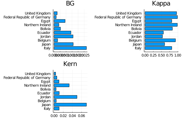
With the fitting complete we can now examine the final parameters. I select 10 random countries out of the 50 the model was fitted and plot there individual parameters.

using Plots
using StatsPlots
sort!(allParams, :Kappa)

plotInds = Int64.(floor.(rand(10) * 50))
paramPlot = Array{Plots.Plot}(undef, 3)
for (i, param) in enumerate((:BG, :Kappa, :Kern))
    paramPlot[i] = bar(allParams[plotInds, :Country], allParams[plotInds, param], orientation = :horizontal, label=:none, title=string(param))
end

plot(vcat(paramPlot)...)

svg

  • Higher background values: the overall rate of terror attack is higher.
  • Higher \(\kappa\) values: the self-exciting jump is higher as each event has $\kappa$ children events.
  • Higher kernel value, \(\beta\): the decay of the terror attack excitement is quicker.

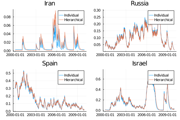
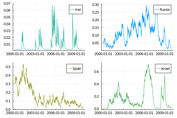
We can also examine the intensity profiles of some countries. If the
intensity is high, the probability of another terror attack is also
high.

selCountrys = ["Iran", "Russia", "Spain", "Israel"]
intPlots = Array{Plots.Plot}(undef, length(selCountrys))
for (i, country) in enumerate(selCountrys)
    subData = @where(allIntensities, :Country .== country, year.(:Date) .>= 2000)
    intPlots[i] = plot(subData.Date, subData.Intensity, label=country,
                       linecolour=Int64(ceil(rand()*10)))
end
plot(vcat(intPlots)...)

svg

For Iran, we can see that the attacks are coming in bursts with periods of down time. Whereas for the other three countries there is a more fluid ebb and flow of the intensity.

The Hierarchical Model

We now turn to fitting the hierarchical model, where there is just one background, $\kappa$ and kernel parameter shared across all the countries. This is a newly implemented feature of my HawkesProcesses package and you can fit a simple Hawkes process with exponential kernel across multiple timeseries in a hierarchical model.

hierParams1 = HawkesProcesses.hierarchical_fit(allEventsTrain, maxT, 5000);
hierParams2 = HawkesProcesses.hierarchical_fit(allEventsTrain, maxT, 5000);
paramEstimates = map(x->mean(x[500:end]), hierParams1)
(0.0011, 0.94, 0.016)

Here we can see that across all countries, each terror attack has on
average 0.94 children terror attack. So they are very self
exciting. From the kernel parameter we can see that this impact lasts
60 days on average.

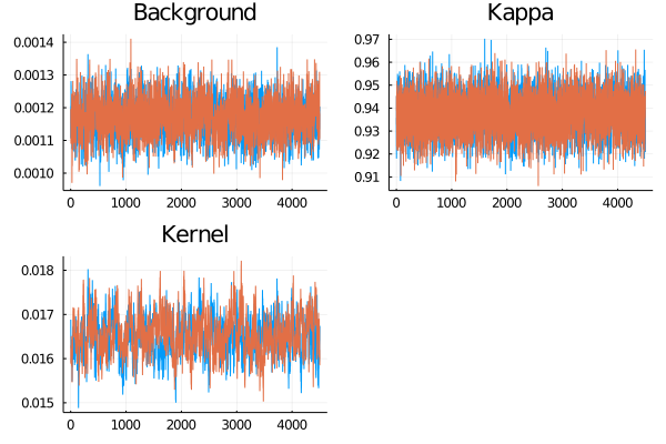
Now all the models I’ve been fitting have been using a Bayesian algorithm, so
we want to assess whether the parameters have converged to the same
value. I’ve fit two chains to also assess the convergence of the model.

bgPlot = plot(hierParams1[1][500:end], title="Background", label=:none)
plot!(bgPlot, hierParams2[1][500:end], label=:none)

kappaPlot = plot(hierParams1[2][500:end], title="Kappa", label=:none)
plot!(kappaPlot, hierParams2[2][500:end], label=:none)

kernPlot = plot(hierParams1[3][500:end], title="Kernel", label=:none)
plot!(kernPlot, hierParams2[3][500:end], label=:none)

plot(bgPlot, kappaPlot, kernPlot)

svg

Everything is looking good.

Now we are happy with the model, we can compare their outputs and see
how they differ.

We will calculate the likelihood and intensity functions. The likelihoods will allow us to perform some model criticism later, whereas the intensity will give us a visual inspection of the model output.

hierIntensities = Array{DataFrame}(undef, length(modelCountries))
hierLikelihood = Array{DataFrame}(undef, length(modelCountries))
for (i, country) in enumerate(modelCountries)
    
  intens = HawkesProcesses.intensity(collect(0:maxT), allEvents[i], 
                                     paramEstimates[1], paramEstimates[2], Exponential(1/paramEstimates[3]))
    hierIntensities[i] = DataFrame(Intensity = intens, t=collect(0:maxT), 
                                   Country=country, Date = collect(minDate:Day(1):maxDate))
    hierLikelihood[i] = DataFrame(HierLikelihoodAll=HawkesProcesses.likelihood(allEvents[i], paramEstimates[1], paramEstimates[2], Exponential(1/paramEstimates[3]), maxT),
                               Country = country,
                               HierLikelihoodTrain = HawkesProcesses.likelihood(allEventsTrain[i], paramEstimates[1], paramEstimates[2], Exponential(1/paramEstimates[3]), maxT))
end

hierIntensities = vcat(hierIntensities...);
hierLikelihood = vcat(hierLikelihood...);

Likelihoods calculated, I can compare the intensities for both models
and see how different they look.

selCountrys = ["Iran", "Russia", "Spain", "Israel"]
intPlots = Array{Plots.Plot}(undef, length(selCountrys))
for (i, country) in enumerate(selCountrys)
    subData = @where(allIntensities, :Country .== country, year.(:Date) .>= 2000)
    subDataHier = @where(hierIntensities, :Country .== country, year.(:Date) .>= 2000)
    p = plot(subData.Date, subData.Intensity, label="Individual", title=country)
    plot!(subDataHier.Date, subDataHier.Intensity, label="Hierarchical")
    intPlots[i] = p
end
plot(vcat(intPlots)...)

svg

Despite the difference in parameters, the final output appear quite similar. Which is reassuring. For Iraq we can see that the hierarchical model decaying slower, but across all countries the spike after each attack is of similar magnitude.

Model Checking

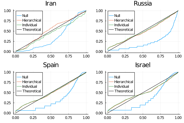
Are terror attacks actually self exciting though? To check for this we
fit a model that doesn’t have any self exciting behaviour and see if
it is better than the Hawkes models.

To check if one model is better than the other, we use the time change
theorem. By using the intensity functions we can transform the event
times and see how close they fall to a straight line. A perfect model
would fall exactly on the straight, a bad model would be far away from
a straight line.

residPlots= Array{Plots.Plot}(undef, length(selCountrys))

for (i, country) in enumerate(selCountrys)
    
   subData = @where(allData, :Country .== country)
   subParams = @where(allParams, :Country .== country)
    
   nullResid = HawkesProcesses.time_change_null(subData.EventTimes, maxT) 
   hierResid = HawkesProcesses.time_change_hawkes(subData.EventTimes, paramEstimates[1], paramEstimates[2], Exponential(1/paramEstimates[3])) 
   indResid = HawkesProcesses.time_change_hawkes(subData.EventTimes, subParams.BG[1], subParams.Kappa[1], Exponential(1/subParams.Kern[1]))
    
   p1 = plot(nullResid[1], nullResid[2], label="Null", title=country)
   plot!(p1, hierResid[1], hierResid[2], label="Hierarchical")
   plot!(p1, indResid[1], indResid[2], label="Individual")
   plot!(0:0.1:1, 0:0.1:1, label="Theoretical", colour="black", legend=:topleft) 
   residPlots[i] = p1
end
plot(residPlots...)

svg

Here we can see that both Hawkes models improve on the model without
self exciting (the null model) as they are closer to the theoretical
straight black line. This suggests there is some notion of self
excitability between the events, which means we can move onto deciding
which Hawkes model is better, the individual or the hierarchical
model?

Model Comparison

How do we know what model is better? I’ve written about deviance
information criteria before
(here) and
it is implemented in this HawkesProcesses package. But I might aswell use this to illustrate other information criteria’s; Bayesian and Akaike. Both are about weighing up the likelihood with the number of parameters in the model. There is an important point to note that these methods are not strictly Bayesian and don’t make full use of the full posterior sampling, but I think it is useful to have a general indicator and comparison between models, even if it isn’t strictly pure. Plus this also highlights the benefits of a Bayesian approach, you can reduce it to a frequentist estimate just by taking your point estimate of the parameters.

By assuming that each country is independent of each other, we arrive at a final likelihood value by summing up each individual likelihood for the country. Then by separating the training set likelihood and total likelihood we can come up with a test set likelihood, which we can use to perform our model comparison.

indLikelihood = @select(allParams, :Country, :LikelihoodAll, :LikelihoodTrain)
allLikelihood = leftjoin(indLikelihood, hierLikelihood, on=:Country)
allLikelihood = @transform(allLikelihood, 
                        LikelihoodTest = :LikelihoodAll - :LikelihoodTrain, 
                        HierLikelihoodTest = :HierLikelihoodAll - :HierLikelihoodTrain)

indAll = sum(allLikelihood.LikelihoodAll)
indTest = sum(allLikelihood.LikelihoodTest)
indTrain = sum(allLikelihood.LikelihoodTrain)

hierAll = sum(allLikelihood.HierLikelihoodAll)
hierTrain = sum(allLikelihood.HierLikelihoodTrain)
hierTest = sum(allLikelihood.HierLikelihoodTest)

allEventsN = sum(map(length, allEvents))
trainEventsN = sum(map(length, allEventsTrain))
testEventsN = allEventsN - trainEventsN

finalResults = vcat(DataFrame(Model = "Ind", 
                              Params = 3*length(modelCountries),
                              Sample = ["All", "Test", "Train"], 
                              Likelihood = [indAll, indTest, indTrain],
                              NEvents = [allEventsN, testEventsN, trainEventsN]),
                    DataFrame(Model = "Hier", 
                              Params = 3,
                              Sample = ["All", "Test", "Train"],  
                              Likelihood = [hierAll, hierTest, hierTrain],
                              NEvents = [allEventsN, testEventsN, trainEventsN])
)

6 rows × 5 columns

Model Params Sample Likelihood NEvents
String Int64 String Float64 Int64
1 Ind 150 All -65332.8 20466
2 Ind 150 Test -18064.0 6163
3 Ind 150 Train -47268.8 14303
4 Hier 3 All -65715.0 20466
5 Hier 3 Test -18023.3 6163
6 Hier 3 Train -47691.8 14303

Here we can see that the individual model has a lower likelihood by around 600. But, it has 150 parameters compared to the hierarchical model that has just 3. We can use Akaike Information Criteria which takes into account the number of parameters.

\[\text{AIC} = 2k – 2\mathcal{L}\]

The better model will have a lower AIC value.

There is also the Bayesian information criteria, which is slightly different in that it also takes into account the number of datapoints.

\[\text{BIC} = k\ln(n) – 2 \mathcal{L}\]

Again, we want the model with the lower BIC.

finalResults = @transform(finalResults, AIC = 2*:Params - 2*:Likelihood)
finalResults = @transform(finalResults, BIC = :Params .* log.(:NEvents) - 2*:Likelihood)
@where(finalResults, :Sample .== "Test")

2 rows × 7 columns

Model Params Sample Likelihood NEvents AIC BIC
String Int64 String Float64 Int64 Float64 Float64
1 Ind 150 Test -18064.0 6163 36427.9 37436.9
2 Hier 3 Test -18023.3 6163 36052.6 36072.7

When we look at just the test set we can see that the likelihood is higher and both the BIC and AIC are lower, which shows the hierarchical model is preferred. Especially since there are just 3 parameters compared to the 150.

The hierarchical model is also preferred as it shows how the model is generalisable to countries not included in the test set. Whereas for the individual model there is no way of using parameters of other countries to apply to a new country.

There is another model that is in between both one set of parameters for all countries and \(3N\) parameters for \(N\) countries and that involves partial pooling, I’ve written about pooling before here and you can take similar ideas and apply them to this applications. It takes a bit more work and is beyond the scope of this blog post, so I will save that for another blog post.

National Security Policy Implications

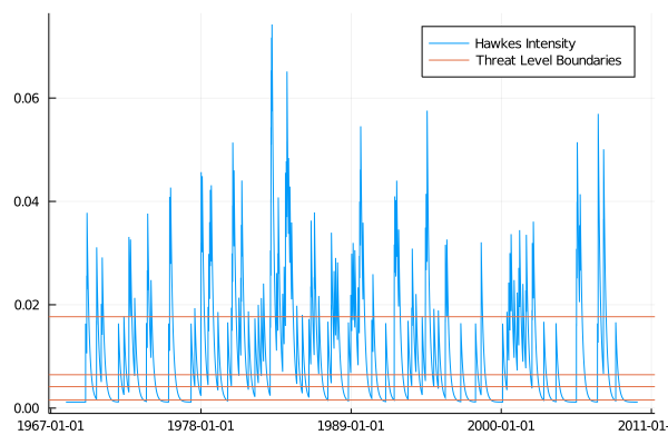
Let’s say you are a government official reading this post and think it is useful but want to know how the Hawkes parameters and structure could be directly incorporated into terror attack responses. In the UK we have threat levels: Low, Moderate, Substantial, Severe and Critical. So we could split up the Hawkes intensity in 5 quantiles, where each quantile occupies one of these levels.

ukIntensity = @where(hierIntensities, :Country .== "United Kingdom")
levls = quantile(ukIntensity.Intensity, [0.2, 0.4, 0.5, 0.8])

plot(ukIntensity.Date, ukIntensity.Intensity, label="Hawkes Intensity")
hline!(levls, label="Threat Level Boundaries")

svg

Each horizontal line represents the boundary between the different threat levels. Each attack causes a move across two boundaries making it quite reactive. As you can see at the end of this dataset we were back into “low” level having not seen an attack in a while.

We can also use the parameters to learn about the structure between events. As it is also a hierarchical model, these interpretations apply to all terror attacks not just those in the UK.

paramEstimates
(0.0011, 0.94, 0.016)

Each terror attack has 0.94 children terror attacks, which is very
high and suggests quite a bit of self-excitation. We can see this
above as each terror attack causes that large spike. Using the kernel
parameter we see that the half-life of the kernel is
\(\frac{1}{0.016} = 62.5\) days. So it takes roughly two months for the
increased intensity to reduce by half. So, after each terror attack
increase readiness for 60 days! It is a shame that the data set is
almost 10 years out of date so we can’t get an to date picture of
where we are right now. If you know of a more recent datasource, please let me know below.

Summary

Quite the chunky blog post and on a heavier subject than what I usually write about, but a nice application of the Hawkes process and how it can be used in this terror attack context. I’ve fitted two Hawkes models and shown that they improve on a null Poisson model, then between the Hawkes models I found that the hierarchical model with the same parameters per country was a better model than one with separate parameters for each country. Potentially, the individual parameter model overfit the data and didn’t generalise to the unseen events. I then has a guess about how the outputs from this type of model could be used to adjust terror related public policy.