First Steps #2: The REPL

By: Josh Day

Re-posted from: https://www.juliafordatascience.com/first-steps-2-the-repl/

Prerequisite

What is the REPL?

First Steps #2: The REPL

REPL stands for Read-Eval-Print-Loop.  When you open Julia (double-click the icon or type julia in a terminal if you have it on your PATH), you'll enter Julia's REPL.  You'll see something like this:

               _
   _       _ _(_)_     |  Documentation: https://docs.julialang.org
  (_)     | (_) (_)    |
   _ _   _| |_  __ _   |  Type "?" for help, "]?" for Pkg help.
  | | | | | | |/ _` |  |
  | | |_| | | | (_| |  |  Version 1.6.0 (2021-03-24)
 _/ |\__'_|_|_|\__'_|  |  Official https://julialang.org/ release
|__/                   |

julia>
Julia REPL at Startup

When you type something and press enter, Julia will take your input, evaluate it, and print the result, e.g. typing x = "Hello" and hitting enter will result in:

julia> x = "Hello"
"Hello"

julia>
x = "Hello"

REPL Modes

Julia's REPL has amazing modes that affect how Julia interprets your input.  Here are the modes that are built-in:

? ➡ Help Mode 📖

Help Mode does a few things, best seen through example.  Type ? to enter Help Mode.  Then type println and press enter.

First Steps #2: The REPL
Image of ?println Output
  • The top line displays a fuzzy search of what you searched for.  This will help you find items even if you mistype something.
  • If your search term matches an existing identifier, the documentation for that identifier will print.  In this example our search found the function println.

Press delete to go back to Julia mode and type x = 1.  Now type ?x.  

  • Your search x matches with the x you just created.  However, there is no documentation available, so a summary of x (its type information) is printed out instead.  We'll talk about types in a future post.

; ➡ Shell Mode 💻

This lets you run shell commands (as if you opened a terminal but didn't start Julia).  A benefit of Julia's Shell Mode is that you can interpolate values into a command with $, e.g.

shell> echo $x
1
Interpolating a Julia value into a Shell Mode command.

] ➡ Pkg Mode 📦

Pkg Mode lets you run commands with Julia's package manager (we'll cover this in-depth in a future post) .  In the previous post we added packages with:

using Pkg

Pkg.add("StatsBase")

Alternatively, we could have used Pkg Mode and entered add StatsBase instead 🎉!  On a fresh install of Julia 1.6 you'll see something like:

(@v1.6) pkg> add StatsBase
    Updating registry at `~/.julia/registries/General`
    Updating git-repo `https://github.com/JuliaRegistries/General.git`
   Resolving package versions...
    Updating `~/.julia/environments/v1.6/Project.toml`
  [2913bbd2] + StatsBase v0.33.4
    Updating `~/.julia/environments/v1.6/Manifest.toml`
  [34da2185] + Compat v3.25.0
  [9a962f9c] + DataAPI v1.6.0
  [864edb3b] + DataStructures v0.18.9
	⋮
  [3f19e933] + p7zip_jll
  Progress [========================================>]  10/10
10 dependencies successfully precompiled in 9 seconds
Using Pkg Mode to Install StatsBase

REPL Modes are extendable! 🔌

Julia packages can add their own REPL modes.  Some examples are:

  • $RCall (interpret input as R)
  • <Cxx (interpret intput as C++)

Notable REPL Features

Re-Run a Line

  • Press the up key to display the previously-run command.  Continue pressing up to go through your history.
  • Press ctrl-r to activate a search of your history.  Begin typing and the most recent line that contains your search will appear.  You can continue pressing ctrl-r to move backwards through matching lines in your history and ctrl-s to move forward.  If you've only run the commands seen in this and the previous post, typing x will then find the x = 1 line you entered earlier.  Press enter to choose the matching line.  

The Value of the Previous Line

The Julia REPL stores the value of the previous line in a variable called ans.  

julia> x = 1
1

julia> ans + 1
2
Using ans

Tab-Completion

You can Auto-complete names, file paths, symbols, and emoji.  

  • Try typing prin and pressing tab.  Your input will change to print.  Now press tab again.  Julia will show you that there are more identifiers available that also match with print.
julia> print
print       println      printstyled
print[TAB]
  • Julia can help you type out file/directory paths when you press tab inside of a string.  For example, suppose you have a file at "/Users/<username>/file.csv". Typing "/Users/<username>/f" and then tab will autocomplete the f to file.csv (if it's the only file/directory that begins with f).  If there are multiple matches, press tab again to display them.
  • Try typing \pi and pressing tab.  Your input will change to π ! 🎉
  • Try typing \:smile: and pressing tab.  Your input will change to 😄!  Fun fact: This feature was introduced as an April Fool's Day joke but won traction in the Julia community.  You can even use emoji as variables!  There's no good reason to do this, but it's neat 🙃.
julia> 😄 = 1
1

julia> 🚀 = 2
2

julia> 😄 + 🚀
3
Emoji variables

Skip Printing

Sometime you may not want to display the return value of a line (e.g. the object prints a wall of text).  You can always skip displaying an object by adding ; to the end of a line:

julia> x = "1234"
"1234"

julia> x
"1234"

julia> x;

julia>
Skip Printing with ;

That's It!

This is a high-level overview of the Julia REPL.  It covers the things you'll need to know to get started with the REPL.  If you want to go further into the weeds, check out the official docs here.

Next up is First Steps #3: Plots.
Additional Resources

Union Find Dicts: Dictionaries Keyed on Equivalence Classes

By: Philip Zucker

Re-posted from: https://www.philipzucker.com/union-find-dict/

Dictionary/map data structures usually have a set-like counter part. You get a Set data structure over the keys of a dict by just storing some dummy value such as ().

  • Inserting element k in the set is dictionary insertion d[k] = ()
  • Key lookup is the same thing as check set membership. haskey(d,k)
  • Set union is dictionary merge.
  • Enumerating elements of the set is enumerating the keys of the dict.

Not every set data structure is derived this way. BitSets for example are not really a dict you ignore the value in.
Nevertheless, hash and binary tree based Maps and Sets have this similarity to each other. They are largely the same except perhaps the set data structure is specialized to not even bothering to hold the default value.

The union find data structure is a way of storing disjoint unions of sets in such a way that the union operation remains fast. There is a pretty good explanation here https://en.wikipedia.org/wiki/Disjoint-set_data_structure

I want a version of union find that is a dictionary that stores values keyed on these equivalence classes. I mention why at the end (spoiler: Egraphs).

I’m kind of surprised this abstract data structure interface is not commonly available. I couldn’t find anything when I looked. It is only a very small addition to the regular union find.

Basic Union Find Without Path Compression

You can find the DataStructures.jl version of the union find data structure with path compression here https://github.com/JuliaCollections/DataStructures.jl/blob/master/src/disjoint_set.jl. It’s pretty readable, which is a nice aspect of Julia.

struct IntDisjointSet
    parents::Vector{Int64}
end

This stores and array of indices of the parents of the nodes.

IntDisjointSet() = IntDisjointSet(Vector{Int64}[])
Base.length(x::IntDisjointSet) = length(x.parents)

Here we use a little trick, perhaps ill advised. When an item j is a root node, the storage at
x.parents[j] is redundant. One choice is to set x.parents[j] = j in this case. This is what the DataStructures.jl version does, and it does make some operations clean. Another is to use this space to store extra information. I used negatives numbers at the parent node pointer to represent the size of the tree. This allows union to easily place the smaller tree under the larger one. Hence creating a set of size 1 has a -1 put in its parents array here.

Base.push!(x::IntDisjointSet) = push!(x.parents, -1)

Here is a simple find_root loop. It traverses up the parent array. Here is a basic version of it where I stripped out path compression. Sacrilege you say? Perhaps. Path compression is kind of the cleverest and most confusing part.

function find_root(x::IntDisjointSet, i::Int64)
    while x.parents[i] >= 0
        i = x.parents[i]
    end
    return i
end

The union operation is almost interesting. It sets the parent of the smaller tree to the larger one. This has a tendency to keep the trees shallow. You could also use the rank of the subtree. In the absence of path compression, the rank is the height.

function Base.union!(x::IntDisjointSet, i::Int64, j::Int64)
    pi = find_root(x, i)
    pj = find_root(x, j)
    if pi != pj
        isize = -x.parents[pi]
        jsize = -x.parents[pj]
        if isize > jsize # swap to make size of i less than j
            pi, pj = pj, pi
            isize, jsize = jsize, isize
        end
        x.parents[pj] -= isize # increase new size of pj
        x.parents[pi] = pj # set parent of pi to pj
    end
    return pj
end

I have some suspicion for a use case that normalizing the parent pointers all at once in a batch might be kind of nice. Then further lookups are no longer mutating and can more easily be done in parallel and without a loop. Depends on your usage pattern.

function normalize!(x::IntDisjointSet)
    for i in length(x)
        pi = find_root(x, i)
        if pi != i
            x.parents[i] = pi
        end
    end
end

# If normalized we don't even need a loop here.
function _find_root_normal(x::IntDisjointSet, i::Int64)
    pi = x.parents[i]
    if pi < 0 # Is `i` a root?
        return i
    else
        return pi
    end
end

A question I had is if it was possible to make a dictionary structure that is keyed on equivalence classes. Yes, it is, With some caveats.

You need to define what you want to happen to the values when two equivalance class keys merge. I think a reasonable requirement is that values held in the are combined using an associative and commutative operation, since you are unlikely to be able to predict these orderings. It is tempting to think that this should be a semilattice (idempotent) but it is not necessary.
If you wanted to use arrays with array concatenation for example, expect the order of the array to be scrambled.

struct IntDisjointMap
    parents::Vector{Int64}
    values::Vector{Any}
    merge_fun
end

IntDisjointMap(merge_fun) = IntDisjointMap(Vector{Int64}[], [], merge_fun)

Most of the previous definitions stay the same. We do have to change the definition of union and we can add new definitions for retrieving and updating the dict.

Base.getindex(x::IntDisjointMap, i::Int64) = x.values[find_root(x,i)]
Base.setindex!(x::IntDisjointMap, v, i::Int64) = x.values[find_root(x,i)] = v


function Base.union!(x::IntDisjointMap, i::Int64, j::Int64)
    pi = find_root(x, i)
    pj = find_root(x, j)
    if pi != pj
        isize = -x.parents[pi]
        jsize = -x.parents[pj]
        if isize > jsize # swap to make size of i less than j
            pi, pj = pj, pi
            isize, jsize = jsize, isize
        end
        x.parents[pj] -= isize # increase new size of pj
        x.values[pj] = x.merge_fun(x.values[pj], x.values[pi])
        x.values[pi] = nothing # clear out unused storage
        x.parents[pi] = pj
    end
    return pj
end

Some usage storing integers in the Map using + as a merge operation

using Test
G = IntDisjointMap(+)
push!(G, 1)
@test G.parents == [-1]
@test G.values == [1]
push!(G,14)
@test G.parents == [-1, -1]
@test G.values == [1, 14]
@test G[1] == 1
@test G[2] == 14
union!(G,1,2)
@test G.parents == [2,-2]
@test G.values == [nothing, 15]
@test G[1] == 15
@test G[2] == 15
push!(G, 4)
@test find_root(G,1) == 2
@test find_root(G,2) == 2
@test find_root(G,3) == 3
union!(G,1,3)
@test G[3] == 19
@test find_root(G,3) == 2
@test find_root(G,1) == 2
@test G.parents == [2,-3,2]

G[3] = 42
@test G[2] == 42

Why?

Well, I think the the IntDisjointMap is a missing obvious intersection of abstract data type interfaces.

I’ve been playing around with EGraphs lately https://www.philipzucker.com/egraph-1/, and they involve a bipartite graph between Equivalence classes and ENodes, which are tern nodes with the children replaced by EClass Ids. A fairly minimal representation of such a structure would be an IntDisjointMap holding ENodes.

struct ENode
    head::Symbol
    args::Vector{Int64}
end

I’m kind of hoping to make a very minimal, perhaps inefficient implementation of the essence of egraphs.

Notes

Structures mapping equivalence classes to terms also show up in unification.

There is no impediment to implementing this interface over a full path compressed union find.
It is also possible to implement this as a wrapper over a normal union find, at the expense of some unnecessary find operations

struct IntDisjointMap
    unionfind::IntDisjointSet
    values::Vector{Int64}
    merge_fun
end

I think that perhaps using Parametric types like so may give a speed boost as Julia specializes on types.

struct IntDisjointMap{V}
    parents::Vector{Int64}
    values::Vector{V}
    merge_fun
end

Even further, putting a tag of the merge_fun in the type might do something good specializing in that function call.

struct IntDisjointMap{V, merge_fun}
    parents::Vector{Int64}
    values::Vector{V}
end

Would Int32 give savings?

Is there a category of Equivalence Maps? Maybe.

How to do this in prolog? A dict keyed on unification variables. Would attributed variables suffice?

Crypto Data using AlphaVantatge.jl

By: Dean Markwick's Blog -- Julia

Re-posted from: https://dm13450.github.io/2021/03/27/CryptoAlphaVantage.html

Julia 1.6 is hot off the press, so I’ve installed it and fired off this quick blog post to give 1.6 a test drive. So far, so good and there is a real decrease now in the latencies in both loading up packages and getting things going.

AlphaVantage have data on cryptocurrencies and not just stocks and fx. Each of which are implemented in AlphaVantage.jl. This is a simple blogpost that takes you through each function and how it might be useful to analyse cryptocurrencies.

Firstly, what coins are available? Over 500 (542 to be precise). Now as a crypto tourist, I’m only really familiar with the most popular ones that are causing the headlines. So I’ve taken the top 10 from coinmarketcap and will use those to demonstrate what AlphaVantage can do.

using AlphaVantage
using Plots
using DataFrames, DataFramesMeta
using CSV, Dates, Statistics

ccys = ["BTC", "ETH", "ADA", "DOT", "BNB", "USDT", "XRP", "UNI", "THETA", "LTC"]

FCAS Health Index from Flipside Crypto

AlphaVantage have partnered with Flipside Crypto to provide their ratings of different coins. This is designed to give some further info on different coins rather than just looking at what recently increased massively.

ratings = crypto_rating.(ccys);

Simple broadcasted call to get the ratings for each of the 10 currencies above. We format the response into a dataframe and get a nice table out. Not all the coins have a rating, so we have to filter out any empty ratings.

inds = findall(.!isempty.(ratings))
ratingsFrame = vcat(map(x->DataFrame(x["Crypto Rating (FCAS)"]), ratings[inds])...)
rename!(ratingsFrame, Symbol.(["Symbol", "Name", "Rating", "Score", "DevScore", "Maturity", "Utility", "LastRefresh", "TZ"]))
for col in (:Score, :DevScore, :Maturity, :Utility)
    ratingsFrame[!, col] .= parse.(Int64, ratingsFrame[!, col])
end
ratingsFrame

7 rows × 9 columns (omitted printing of 1 columns)

Symbol Name Rating Score DevScore Maturity Utility LastRefresh
String String String Int64 Int64 Int64 Int64 String
1 BTC Bitcoin Superb 910 868 897 965 2021-03-26 00:00:00
2 ETH Ethereum Superb 973 966 896 997 2021-03-26 00:00:00
3 ADA Cardano Superb 964 969 931 966 2021-03-26 00:00:00
4 BNB Binance Coin Attractive 834 745 901 932 2021-03-26 00:00:00
5 XRP XRP Attractive 842 881 829 794 2021-03-26 00:00:00
6 THETA THETA Caution 588 726 915 353 2021-03-26 00:00:00
7 LTC Litecoin Attractive 775 652 899 905 2021-03-26 00:00:00

Three superb, three attractive and one caution. THETA gets a lower utility score which is dragging down its overal rating. By the looks of it, THETA is some sort of streaming/YouTube-esque project, get paid their token by giving your excess computing power to video streams. There website is here and I’ll let you judge whether they deserve that rating.

To summarise briefly each of the ratings is on a 0 to 1000 scale in three different areas:

  • Developer Score (DevScore)

Things like code changes, improvements all taken from the repositories of the coins.

  • Market Maturity (Maturity)

This looks at the market conditions around the coin, so things like liquidity and volatility.

  • User Activity (Utility)

On chain activities, network activity and transactions, so is the coin being used for something actually useful. Hence why you can see why ETH is ranked the highest here.

More details are on their website here.

Timeseries Data

AlphaVantage also offer the usual time series data at daily, weekly and monthly frequencies. Hopefully you’ve read my other posts (basic market data and fundamental data), so this is nothing new!

Now for each 10 tokens we can grab their monthly data and calculate some stats and plot some graphs.

monthlyData = digital_currency_monthly.(ccys[inds], datatype = "csv");

Again formatting the returned data into a nice dataframe gives us a monthly view of the price action for each of the currencies. I format the date column, calculate the monthly log return and cumulative log return.

function format_data(x, ccy)
    df = DataFrame(x[1])
    rename!(df, Symbol.(vec(x[2])), makeunique=true)
    df[!, :timestamp] = Date.(df[!, :timestamp])
    sort!(df, :timestamp)
    df[!, :Return] = [NaN; diff(log.(df[!, Symbol("close (USD)")]))]
    df[!, :CumReturn] = [0; cumsum(diff(log.(df[!, Symbol("close (USD)")])))]
    df[!, :Symbol] .= ccy
    df
end

prices = vcat(map(x -> format_data(x[1], x[2]), zip(monthlyData, ccys[inds]))...)
first(prices, 5)

5 rows × 14 columns (omitted printing of 7 columns)

timestamp open (USD) high (USD) low (USD) close (USD) open (USD)_1 high (USD)_1
Date Any Any Any Any Any Any
1 2018-08-31 7735.67 7750.0 5880.0 7011.21 7735.67 7750.0
2 2018-09-30 7011.21 7410.0 6111.0 6626.57 7011.21 7410.0
3 2018-10-31 6626.57 7680.0 6205.0 6371.93 6626.57 7680.0
4 2018-11-30 6369.52 6615.15 3652.66 4041.32 6369.52 6615.15
5 2018-12-31 4041.27 4312.99 3156.26 3702.9 4041.27 4312.99
returnPlot = plot(prices[!, :timestamp], prices[!, :CumReturn], group=prices[!, :Symbol],
                  title="Cummulative Return",
                  legend=:topleft)
mcPlot = plot(prices[!, :timestamp], 
              prices[!, Symbol("market cap (USD)")] .* prices[!, Symbol("close (USD)")], 
              group=prices[!, :Symbol],
              title="Market Cap",
              legend=:none)

plot(returnPlot, mcPlot)

svg

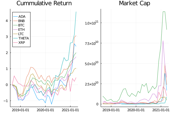
There we go, solid cumulative monthly returns (to the moon!) but bit of a decline in market cap recently after a week of negative returns. If you want higher frequencies there is always

  • digital_currency_daily
  • digital_currency_weekly

which will return the same type of data, just indexed differently.

Is the Rating Correlated with Monthly Trading Volume?

We’ve got two data sets, now we want to see if we can explain some the crypto scores with how much is traded each month. For this we simply take the monthly data, average the monthly volume traded and join it with the ratings dataframe.

gdata = groupby(prices, :Symbol)
avgprices = @combine(gdata, MeanVolume = mean(:volume .* cols(Symbol("close (USD)"))))
avgprices = leftjoin(avgprices, ratingsFrame, on=:Symbol)

7 rows × 10 columns (omitted printing of 2 columns)

Symbol MeanVolume Name Rating Score DevScore Maturity Utility
String Float64 String? String? Int64? Int64? Int64? Int64?
1 BTC 2.473e10 Bitcoin Superb 910 868 897 965
2 ETH 9.6248e9 Ethereum Superb 973 966 896 997
3 ADA 2.6184e9 Cardano Superb 964 969 931 966
4 BNB 3.7598e9 Binance Coin Attractive 834 745 901 932
5 XRP 3.28003e9 XRP Attractive 842 881 829 794
6 THETA 6.36549e8 THETA Caution 588 726 915 353
7 LTC 1.71448e9 Litecoin Attractive 775 652 899 905

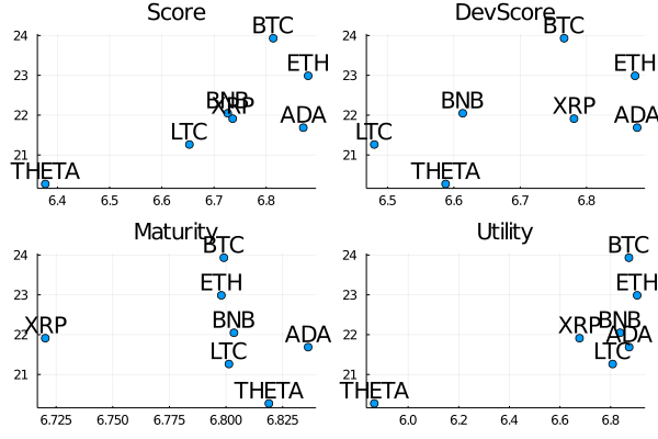
Visually, lets just plot the different scores on the x-axis and the monthly average volume on the y-axis. Taking logs of both variables stops BTC dominating the plots.

scorePlots = [plot(log.(avgprices[!, x]), 
                   log.(avgprices.MeanVolume), 
                   seriestype=:scatter, 
                   series_annotations = text.(avgprices.Symbol, :bottom),
                   legend=:none, 
                   title=String(x)) 
    for x in (:Score, :DevScore, :Maturity, :Utility)]
plot(scorePlots...)

svg

Solid linear relationship in the score and dev score metrics, not so much for the maturity and utility scores. Of course, as this is a log-log plot a linear relationship indicates power law behaviour.

Side note though, the graphs are a bit rough around the edges, labels are overlapping and even crossing though the axis. Julia needs a ggrepel equivalent.

Summary

Much like the other functions in AlphaVantage.jl everything comes through quite nicely and once you have the data its up to you to find something interesting!