Julia GPU Programming with WSL2

By: Fabian Becker

Re-posted from: https://geekmonkey.org/julia-gpu-programming-with-wsl2/

Julia GPU Programming with WSL2

I use Windows for gaming. It's been a long time since I've last done any serious development work on my Windows machine and yet I still spent a good chunk of money on building out a beefy machine for my efforts to learn machine learning. It has taken me a few months to finally sit down and get this machine ready for anything other than gaming.

With the recent announcement of GUI support for WSLg I got really excited to try out WSL and see how good the GPU support actually is, but that's not the main reason. I've been shying away from developing on Windows because I'm used to a *NIX environment. WSL gives you that, but up until recently you wouldn't have been able to interact with any GPU – and this all changed with this announcement!

You can watch the video below to see what's coming for WSL2.

The first half of this article will show you how to get everything set up and in the second half we'll set up CUDA.jl in Julia. Since the latter part is about CUDA I'll assume that you have a compatible nVidia GPU.

Installation

Here's a summary of what we need to go through to prepare our environment:

  • Update Windows 10 to latest release on the dev channel
  • Install nVidia CUDA drivers
  • Install Ubuntu 20.20 in WSL2
  • Install Linux CUDA packages
  • 🎉

Windows 10 Insider Preview

At the time of writing all of the features are only available through the Windows Insider Program. The Windows Insider Program allows you to receive new Windows features before the hit the main update line. The program is split into three channels: Dev, Beta and Release Preview.

To receive the update with WSLg and GPU support we will need to switch to the dev channel.

Julia GPU Programming with WSL2

Note: The dev channel comes with some rough edges and potential for system instability. Be mindful of this when you switch and make sure you have backups!

After installing all downloaded updates you should end up with OS Build 21364 or higher. You can check your OS Build by running winver in PowerShell/cmd.

Julia GPU Programming with WSL2
Run winver using the Windows Run command

With this all set we can hop on to install the latest WSL2 compatible CUDA drivers.

CUDA drivers

NVIDIA are providing special CUDA drivers for Windows 10 WSL. The link below will take you to the download page. It's required to sign up for the NVIDIA Developer Program, which is free.

GPU in Windows Subsystem for Linux (WSL)
CUDA on Windows Subsystem for Linux (WSL) – Public Preview Microsoft Windows is a ubiquitous platform for enterprise, business, and personal computing systems. However, industry AI tools, models, frameworks, and libraries are predominantly available on Linux OS. Now all users of AI – whether they ar…
Julia GPU Programming with WSL2

Follow the setup wizard (I chose the express installation which keeps existing settings in place).

Note: There's also a documentation page provided by NVIDIA around setting up your GPU for WSL. I found the docs to be outdated and not working on my machine.

Installing Ubuntu 20.04 LTS with WSL2

Before we can proceed with installing Ubuntu I advise to update the WSL kernel by running:

wsl --update

In case you're like me and don't enjoy the default terminal Windows comes with I suggest you install Windows Terminal from the Microsoft Store. This terminal comes is a lot more pleasant to use than either cmd or the PowerShell terminal ever were.

It's also a good idea to set WSL to default to version 2:

wsl --set-default-version 2

Finally let's install Ubuntu with:

wsl --install --distribution Ubuntu-20.04

In case you were wondering what other distributions are available you can simply run: wsl --list --online.

Ubuntu 20.04 LTS

With Ubuntu installed we have a couple of final steps. First we will add an upstream repo to apt for getting the latest CUDA builds directly from NVIDIA:

sudo add-apt-repository "deb https://developer.download.nvidia.com/compute/cuda/repos/ubuntu2004/x86_64/ /"
Add CUDA apt repository for Ubuntu 20.04

We also need to add NVIDIA's GPG key for the apt repo:

sudo apt-key adv --fetch-keys https://developer.download.nvidia.com/compute/cuda/repos/ubuntu2004/x86_64/7fa2af80.pub 
Add nVidia gpg key

And finally to make sure that we prefer the packages provided by NVIDIA over packages in mainline Ubuntu we need to pin the apt repo:

wget https://developer.download.nvidia.com/compute/cuda/repos/ubuntu2004/x86_64/cuda-ubuntu2004.pin
sudo mv cuda-ubuntu2004.pin /etc/apt/preferences.d/cuda-repository-pin-600
Pin file to prioritize CUDA apt repository

With this out of the way, we're ready to install the CUDA drivers inside our WSL Ubuntu installation:

 sudo apt update && sudo apt install -y cuda-drivers

In case setting up WSL2 with GPU support was all you wanted to do – we're done!

Julia + WSL2 + Cuda.jl

Ok, so as promised in the headline we're now going to install Julia inside our Ubuntu 20.04 and set up Cuda.jl.

Install Julia

At the time of writing Julia 1.6.1 is the latest version available (make sure to check for updates on Julia's download page).

First let's fetch the latest Julia tarball:

wget https://julialang-s3.julialang.org/bin/linux/x64/1.6/julia-1.6.1-linux-x86_64.tar.gz

Extract the .tar.gz:

tar -xvzf julia-1.6.1-linux-x86_64.tar.gz

Move the extracted folder to /opt:

sudo mv -r julia-1.6.1 /opt/

Finally, create a symbolic link to julia inside the /usr/local/bin folder:

sudo ln -s /opt/julia-1.6.1/bin/julia /usr/local/bin/julia

You may pick a different target directory for your installation of Julia or use a version manager like asdf-vm.

Install Cuda.jl

At this point simply run julia in your terminal and you should be dropped into the Julia REPL. I assume you've worked with Julia before and know how to operate it's package manager.

Hit ] to enter pkg mode and install CUDA with:

activate --temp
add CUDA

From here hit backspace and import CUDA. CUDA.jl provides a useful function called functional which will confirm that we've done everything right (well, that's the hope at least, right?).

using CUDA
CUDA.functional()
Julia GPU Programming with WSL2
Ensuring Julia CUDA.jl is functional inside WSL2

You can additionally run CUDA.versioninfo() to get a more detailed breakdown of the supported features on your GPU.

At this point you should have a working installation with WSL2, Ubuntu 20.04, Julia and CUDA.jl. In case you're new to CUDA.jl I suggest you follow the excellent introduction to GPU programming by JuliaGPU or jump in at the deep end with FluxML's GPU support.


If you like articles like this one, please consider subscribing to my free newsletter where at least once a week I send out my latest work covering Julia, Python, Machine Learning and other tech.

You can also follow me on Twitter.
Gaussian processes and linear regression

By: Oisin Fitzgerald

Re-posted from: https://oizin.github.io/posts/gp-linear/index.html

Gaussian processes and linear regression

Oisín Fitzgerald, May 2021

A look at section 6.4 of:

Bishop C.M. (2006). Pattern recognition and machine learning. Springer.

https://www.microsoft.com/en-us/research/publication/pattern-recognition-machine-learning/

Basically this post goes through (Bayesian) linear regression from a Gaussian process space point of view with some example Julia code to make things concrete.

Update (10/11/2021): Deleted "estimating the hyperparameters" section for now as it was too short and had no examples.

Overview

The dominant approach to solving regression problems in machine learning today is finding the parameters \(w\) of a model \(M_w\) that minimise a loss function \(L\) by optimally combining a set of basis vectors. These basis vectors can be the original data \(x_n\) or some transformation \(z_n = \phi(x_n)\) where \((y_n,x_n)\) is the \(n^{th}\) output-input pair \(n \in \{1,…,N\}\) and \(x_n\) is length \(p\) (the number of features). For example:

  • Linear regression: find the best set of weights \(w\) that minimise mean square error \(\left\Vert Y – X w \right\Vert\) giving us predictions \(y_n = w^t x_n\).

  • Deep learning: at the other extreme of complexity we can think of deep learning as learning both the basis vectors and the weights. In a network with \(L\) layers the outputs and weights of the final layer are \(z_L\) and \(w_L\) giving us \(y_n = w_L^t z_L(x_n)\).

With Gaussian processes with are going to switch from thinking in terms of locating which parameters are most likely to have generated the data to considering the data a finite sample from a function that has particular properties. The parameters and function space viewpoint are not conflicting, for example for linear regression:

  1. Parameter space view: \(y\) is a combination of basis functions with the weights being from a mltivariate normal distribution.

  2. Function space view: \(y(x_n)\) is a sample from a family of functions where any finite sample of points \(\{y_1,…,y_N\}\) follow a multivariate normal distibution.

From the parameter to function space view

To fully see the connection let's go from the parameter space view to the function space view for linear regression. The model is

\[y(x_n) = w^t x_n\]

In matrix form the above is written as \(Y = X w\), with each row of the \(N \times p\) matrix \(X\) made up of the \(N\) individual observations \(x^t_n\), each a vector of length \(p+1\), the number of features plus one (to have an intercept term). The prior distribution on our weights \(w\) reflects a lack of knowledge about the process

\[w \sim N(0,\alpha^{-1}I)\]

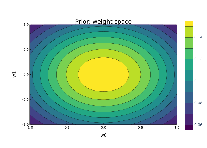
For example if there is one input we have \(w = (w_0, w_1)^t\) and setting \(\alpha = 1.0\) (arbitrarily) the prior looks like the graph below.

using Plots, Random, Distributions, LinearAlgebra
plotlyjs()
Random.seed!(1)
α = 1.0
d = MvNormal([0,0], (1/α)*I)
W0 = range(-1, 1, length=100)
W1 = range(-1, 1, length=100)
p_w = [pdf(d, [w0,w1]) for w0 in W0, w1 in W1]
contourf(W0, W1, p_w, color=:viridis,xlab="w0",ylab="w1",title="Prior: weight space")

Since we treat input features (the x's) as constants this implies a prior distribution for the output

\[y \sim N(0,\alpha X^t X)\]

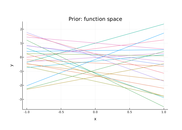
From the function space view we can randomly sample functions at finite spacings \(\mathfrak{X} = \{x_1,…,x_N\}\) from the prior.

Random.seed!(1)
x1 = range(-1, 1, length=100)
X = [repeat([1],100) x1]
d = MvNormal(repeat([0],100), (1/α)*X*transpose(X) + 1e-10*I)
p = plot(x1,rand(d),legend=false,seriestype=:line,title="Prior: function space",xlabel="x",ylabel="y")
for i in 1:20
    plot!(p,x1,rand(d),legend=false,seriestype=:line)
end

The matrix \(K = \text{cov}(y) = \alpha^{-1} X^t X\) is made up of elements \(K_{nm} = k(x_n,x_m) = \frac{1}{\alpha}x_n^t x_m\) with \(k(x,x’)\) the kernel function. Notice that the kernel function \(k(x,x’)\) returns the variance for \(x = x’\) and covariance between \(x\) and \(x’\) otherwise. Also that we are talking here about the covariance between observations, not features. \(K\) is a \(N \times N\) matrix and so can be quite large. There are many potential kernel functions other than \(k = x^tx\) but that's for another day.

Modelling data with straight lines

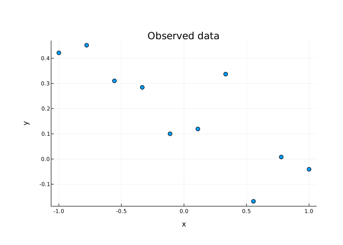
We have a prior on \(y\) and then we observe some data. Let assume there is noise in the data so we observe

\[t_n = y(x_n) + \epsilon_n\]

with \(\epsilon_n \sim N(0,\beta)\) random noise that is independent between observations and \(t = \{t_1,…,t_N\}\) the observed output values for input features \(x_n\).

Random.seed!(1)
n = 10
x1 = range(-1, 1, length=n)
X = [repeat([1],n) x1]
β = 0.01
d = MvNormal(repeat([0],n), (1/α)*X*transpose(X) + β*I)
y = rand(d) 
p = scatter(x1,y,legend=false,title="Observed data",xlabel="x",ylabel="y")

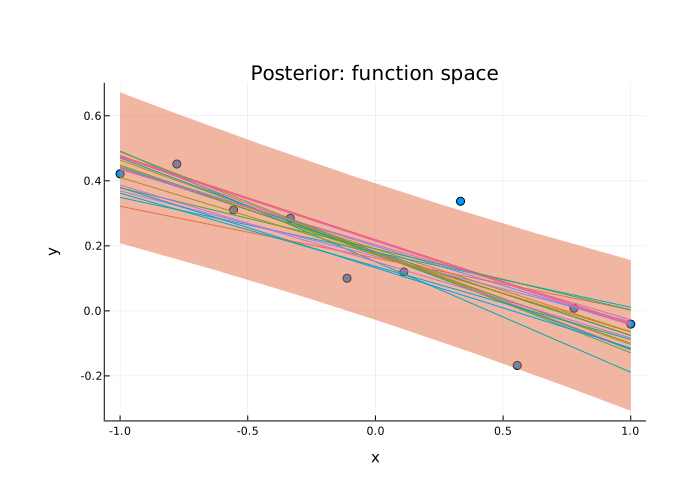
At this point in practise we could estimate the noise parameter \(\beta\), but lets come back to that. For now assume we know that \(\beta = 0.01\). It is worth remember there are no weights giving us the intercept, slope etc but we can sample from our distribution of \(y|t\) or \(t*|t\) or given the observed data. Because our interest is in predicting for new observations we'd like to estimate the posterior \(p(t*|t,x,x*)\) for any future input \(x*\). It turns out the posterior for for any \(t*\) is another normal distribution which is coded below.

p = scatter(x1,y,legend=false,
            title="Posterior: function space",xlabel="x",ylabel="y")# new X's over which to predict
xs = range(-1, 1, length=100)
Xs = [repeat([1],100) xs]
ys = zeros(100)# get ready to construct posterior
σ2 = zeros(100)
C = (1/α)*X*transpose(X) + β*I
Cinv = inv(C)# one prediction at a time 
for i in 1:100
    k = X * Xs[i,:]
    c = Xs[i,:]' * Xs[i,:] + β
    ys[i] = (k' * Cinv) * y
    σ2[i] = c - (k' * Cinv) * k
end
plot!(p,xs,ys, ribbon=(2*sqrt.(σ2),2*sqrt.(σ2)), lab="estimate")
plot!(p,xs,ys)# noise free samples from the posterior
# all predictions at once
m = (Xs * X') * Cinv * y
CV = (Xs * Xs') - (Xs * X') * Cinv * (X * Xs')
CV = Symmetric(CV) + 1e-10*I
d = MvNormal(m, Symmetric(CV) + 1e-10*I)
for i in 1:20
    plot!(p,xs,rand(d),legend=false,seriestype=:line)
end

The order of join and grouping result in DataFrames.jl

By: Blog by Bogumił Kamiński

Re-posted from: https://bkamins.github.io/julialang/2021/04/30/roworder.html

Introduction

Today I want to focus on an issue that is often not noticed by users when
working DataFrames.jl, but in some cases it it might be relevant.

The subject is the order of join and grouping operations result in
DataFrames.jl. The key point of the post is that this order depends on several
factors, so it is simplest to assume that it is undefined.
I am not going to list all cases in my examples, but just focus on showing
the fact as in the future the order might change.

In this post I am using Julia 1.6.1 and DataFrames.jl 1.0.1.

Joins

Consider the following example of innerjoin:

julia> using DataFrames

julia> df1 = DataFrame(x=[2, 3, 1, 4], id1=1:4)
4×2 DataFrame
 Row │ x      id1
     │ Int64  Int64
─────┼──────────────
   1 │     2      1
   2 │     3      2
   3 │     1      3
   4 │     4      4

julia> df2 = DataFrame(x=[1, 3, 2, 5, 6], id2=1:5)
5×2 DataFrame
 Row │ x      id2
     │ Int64  Int64
─────┼──────────────
   1 │     1      1
   2 │     3      2
   3 │     2      3
   4 │     5      4
   5 │     6      5

julia> innerjoin(df1, df2, on=:x)
3×3 DataFrame
 Row │ x      id1    id2
     │ Int64  Int64  Int64
─────┼─────────────────────
   1 │     1      3      1
   2 │     3      2      2
   3 │     2      1      3

julia> innerjoin(df2, df1, on=:x)
3×3 DataFrame
 Row │ x      id2    id1
     │ Int64  Int64  Int64
─────┼─────────────────────
   1 │     1      1      3
   2 │     3      2      2
   3 │     2      3      1

As you can see currently the row order in the result of innerjoin is taken
from the longer table.

Now consider outerjoin (similar results are for leftjoin and rightjoin):

julia> outerjoin(df1, df2, on=:x)
6×3 DataFrame
 Row │ x      id1      id2
     │ Int64  Int64?   Int64?
─────┼─────────────────────────
   1 │     1        3        1
   2 │     3        2        2
   3 │     2        1        3
   4 │     4        4  missing
   5 │     5  missing        4
   6 │     6  missing        5

julia> outerjoin(df2, df1, on=:x)
6×3 DataFrame
 Row │ x      id2      id1
     │ Int64  Int64?   Int64?
─────┼─────────────────────────
   1 │     1        1        3
   2 │     3        2        2
   3 │     2        3        1
   4 │     5        4  missing
   5 │     6        5  missing
   6 │     4  missing        4

Now we have the following parts of the table: first comes the chunk
matching what innerjoin produces, then we have a non-matching part from the
left table, and finally we have a non-matching part from the right table.

While before 1.0 release we did not guarantee the row order in joins, the
actual order has changed in DataFrames.jl 1.0. The reason were performance
considerations. Consider the following examples of joins and their timing:

julia> df1 = DataFrame(x=string.(1:10^7));

julia> df2 = DataFrame(x=string.(1:10));

julia> @time innerjoin(df1, df2, on=:x);
  0.246627 seconds (176 allocations: 13.797 KiB)

julia> @time innerjoin(df2, df1, on=:x);
  0.237981 seconds (175 allocations: 13.781 KiB)

(I am showing you the timings after compilationp; I use Vector{String} to join
on as this case is the slowest scenario under DataFrames.jl 1.0).

Now switch to DataFrames.jl 0.22.7 for a while (you need a fresh session and a
fresh project environment to test this; timings are again after compilation):

julia> df1 = DataFrame(x=string.(1:10^7));

julia> df2 = DataFrame(x=string.(1:10));

julia> @time innerjoin(df1, df2, on=:x);
  0.350317 seconds (177 allocations: 152.602 MiB)

julia> @time innerjoin(df2, df1, on=:x);
  1.140921 seconds (183 allocations: 662.071 MiB)

As you can see the current algorithm not only uses much less memory, but also
it is faster in general and not affected by the argument order (the last thing
was a major bane of joins before 1.0 release of DataFrames.jl).

For a reference check what data.table in R offers in this case in terms of
performance (I am adding it as the performance against data.table is a hot
topic recently):

> library(data.table)
data.table 1.14.0 using 4 threads (see ?getDTthreads).  Latest news: r-datatable.com
> dt1 <- data.table(x=as.character(1:10^7))
> dt2 <- data.table(x=as.character(1:10))
> system.time(merge(dt1, dt2, all=FALSE))
   user  system elapsed
  7.445   0.153   3.544
> system.time(merge(dt1, dt2, all=FALSE, sort=FALSE))
   user  system elapsed
  6.735   0.128   2.827

(note that I have used non-pooled vectors in both cases, as this was the scenario
that allowed me to compare DataFrames.jl 1.0 and 0.22.7 best; clearly if we
joined on pooled vectors the timings would be much better)

Grouping

In groupby operation the rules of ordering of the GroupedDataFrame object
depend on the type of the column you join on (I am assuming you are not passing
sort=true keyword argument, as then groups are sorted). The two cases are:

  • if you join on columns that are pooled (like PooledVector or
    CategoricalVector) and the number of possible groups is not huge
    then you get your result in the order of levels in the pool;
  • otherwise the group ordering is their order of appearance in the source vector.

Here a particular corner case are integer columns, which are treated to be
pooled (so the groups are sorted), unless the range of the integers is huge
(as then we fall back to the order of appearance). Here is an example:

julia> df = DataFrame(x=[3, 1, 2], y=[300, 1, 2])
3×2 DataFrame
 Row │ x      y
     │ Int64  Int64
─────┼──────────────
   1 │     3    300
   2 │     1      1
   3 │     2      2

julia> keys(groupby(df, :x))
3-element DataFrames.GroupKeys{GroupedDataFrame{DataFrame}}:
 GroupKey: (x = 1,)
 GroupKey: (x = 2,)
 GroupKey: (x = 3,)

julia> keys(groupby(df, :y))
3-element DataFrames.GroupKeys{GroupedDataFrame{DataFrame}}:
 GroupKey: (y = 300,)
 GroupKey: (y = 1,)
 GroupKey: (y = 2,)

What is considered to be huge is left undefined (as it might change in the
future), but in general if there is less levels than the number of rows in of
the data frame (this is a typical case in practice) then we do not consider
it as a huge number.

Again – let us do some benchmarking against the 0.22.7 release of DataFrames.jl.
First the results for DataFrames.jl 1.0:

julia> df = DataFrame(x=1:10^7+1, y=[1:10^7; 10^10]);

julia> @time groupby(df, :x);
  0.055407 seconds (64 allocations: 85.834 MiB)

julia> @time groupby(df, :y);
  0.895716 seconds (50 allocations: 280.591 MiB)

and now under 0.22.7 release:

julia> df = DataFrame(x=1:10^7+1, y=[1:10^7; 10^10]);

julia> @time groupby(df, :x);
  0.890674 seconds (31 allocations: 280.590 MiB)

julia> @time groupby(df, :y);
  0.884177 seconds (31 allocations: 280.590 MiB)

As you can see, in the case of grouping integer columns we are much faster
than before if the integer range is not huge.

Let us have a comparison with data.table again (we need to also perform some
aggregation to match apples to apples in terms of timing).

First DataFrames.jl 1.0:

julia> df = DataFrame(x=1:10^7+1, y=[1:10^7; 10^10]);

julia> @time combine(groupby(df, :x), nrow);
  0.180592 seconds (261 allocations: 324.266 MiB)

julia> @time combine(groupby(df, :y), nrow);
  1.006619 seconds (247 allocations: 519.023 MiB)
> df <- data.table(x=1:(10^7+1), y=c(1:10^7, 10^10))
> system.time(df[, .N, by = x])
   user  system elapsed
  0.644   0.088   0.266
> system.time(df[, .N, by = y])
   user  system elapsed
  0.991   0.096   0.404

This time for the huge range DataFrames.jl is slower. (note that data.table
is using four threads – which is great – and I tested my code on a single thread
in Julia, as in DataFrames.jl we do not support multi-threading in this
particular case yet)

Conclusions

In summary: although there are precise rules that determine the order of join
and grouping results is simplest to assume that it is undefined (like in data
bases). The reason for this are operation performance considerations (so the
rules are complex and might change in the future).

However, based on the user feedback, we might in the future consider adding some
keyword arguments to joins or groupby that would guarantee some particular
order. Therefore if you have any thoughts on it please open an issue in
DataFrames.jl repository on GitHub.