It’s that time of year again! Just like last year, I’ll be posting my solutions
to the Advent of Code puzzles. This year, I’ll be
solving the puzzles in Julia. I’ll post my solutions
and code to GitHub as well.
I had a blast with AoC last year, first in R, then as a set of exercises for
learning Rust, so I’m really excited to see what this year’s puzzles will bring.
If you haven’t given AoC a try, I encourage you to do so along with me!
While today’s input format isn’t super complicated, we’ll be doing a good amount
of parsing and manipulating that input, so it makes sense to ingest it as an
efficient data type. I’ve found that working with Tuples generally results in
faster code than using structs, where it makes sense. Since we know how many
values we’ll have in each input record, we can use NTuples for each part.
const SignalPatterns =NTuple{10,String}
const RawOutputs =NTuple{4,String}
const RawInput =@NamedTuple {patterns::SignalPatterns, outputs::RawOutputs}
function parseline(s::AbstractString)::RawInput (patternstr, outputstr) = split(s, " | ")
sortstr = join ∘ sort ∘ collect
patterns =Tuple([sortstr(s) for s in split(patternstr)])
outputs =Tuple([sortstr(s) for s in split(outputstr)])
return (patterns = patterns, outputs = outputs)
endfunction ingest(path)
return open(path) do f
[parseline(s) for s in readlines(f)]
endend
Part One – Easy Street
Today’s puzzle has us decoding scrambled seven-segment displays. Quite frankly,
I’m appalled at the missed opportunity to have this be Day 7’s puzzle, but you
don’t always get what you want, as a wise man once said. It looks like our
submarine has, like, a bajillion of these seven segment displays, each displaying
four digits of pure chaotic garbage at the moment, and our job is to unscramble
them. Well, that’s probably our job in part two. Our job in part one is just to
figure out how many times the numbers 1, 4, 7, and 8 appear in our
display outputs. This is somewhat easy, because each of these numbers contains
a unique count of the seven segments, like so:
All other numbers, it turns out, are represented by either five or six segments.
So, for this part, we just look over all the output values (the ones to the
right of the | in the puzzle input), and count the number of strings of
length 2, 4, 3, or 8.
# Given a `RawOutput` (a Tuple of letter combinations), identify which# ones represent a number containing a unique number of segments, and# just count how many you found.function counteasydigits(outputs::RawOutputs)::Int easyfilter(output) = filter(x -> length(x) in [2, 3, 4, 7], output)
(outputs
|> easyfilter
|> length)
end# Search for the obvious number displays in our outputs and count the# number found.function part1(input)
tooutputs(RI) = map(x -> x.outputs, RI)
easycount(input) = map(counteasydigits, input)
(input
|> tooutputs
|> easycount
|> sum)
end
So, that wasn’t too difficult. In fact, it was almost suspiciously easy…
Part Two – Set Me Up
Now we’re paying for the relatively simple part one, and to be honest, we
definitely should have seen this one coming. Now our main job is to decode the
rest of the signals to identify which combination of letters corresponds to each
display of a particular number. To do this, we’ll compare the letters corresponding
to the segments in the display of known numbers (1, 4, 7, 8) to the letters
corresponding to the segments in the display of unknown numbers (0, 2, 3, 5, 6, 9)
to deduce the unknown numbers. We know how many segments are in each of the
unknown number displays (5 segments -> 2, 3, 5; 6 segments -> 0, 6, 9), so
armed with these known lengths and our four known collections of segments, we
can deduce the remaining numbers. In our solution below, we start with the 5-length
signals, then move on to the 6-length signals. For your reference, here are
the segment arrangements that represent the rest of the numbers:
One example of our approach is identifying the segments that represent the
number 3. Of the 5-segment combinations, only 3 contains all the segments
from the display of 1. Using rules like this for all 6 of the unknown numbers
allows us to identify them and get the problem solution, which is to use our
known signal -> number mapping to get the total value of each of the outputs
and sum them together to solve the puzzle.
function decode(rawinput::RawInput)::Int (patterns, outputs) = rawinput
# Sort the patterns such that the unique patterns are placed in the front# by length, and the non-unique patterns are sorted to the back. sortpatternsby(x) = length(x) in [5, 6] ? length(x) +5: length(x)
sortedpatterns = sort(collect(patterns), by = sortpatternsby)
# These are the easy matches, sorted to the front of # sortedpatterns by our sorting function patternmatches = [
(sortedpatterns[1], 1),
(sortedpatterns[2], 7),
(sortedpatterns[3], 4),
(sortedpatterns[4], 8)
]
# Match the 5- and 6-length patterns (one, seven, four) = sortedpatterns[1:3]
fivecharmatches = getfivecharmatches(sortedpatterns[5:7], four, seven)
sixcharmatches = getsixcharmatches(sortedpatterns[8:10], four, seven)
append!(patternmatches, fivecharmatches, sixcharmatches)
# Now with all the patterns deciphered, let's get the # values in our outputs patterndict =Dict(patternmatches)
numbers = reverse([patterndict[output] for output in outputs])
return sum(numbers[i] *10^(i -1) for i =1:length(numbers))
endfunction getfivecharmatches(patterns, four, seven)::Vector{Tuple{String,Int}}
matches = []
# Use a set of letters representing the segments left if you "subtract"# the segments in seven from the segments in four to help find the # length 5 displays fournotseven = setdiff(four, seven)
# Rules to identify two, three, and five istwo(x) = seven ⊈ x && fournotseven ⊈ x
isthree(x) = seven ⊆ x
isfive(x) = fournotseven ⊆ x
# Check each length 5 set of segments and identify two, three, and fivefor pattern in patterns
match = istwo(pattern) ? (pattern, 2) : isthree(pattern) ? (pattern, 3) : isfive(pattern) ? (pattern, 5) : missing
ismissing(match) && error("Could not match pattern $pattern")
push!(matches, match)
endreturn matches
endfunction getsixcharmatches(patterns, four, seven)::Vector{Tuple{String,Int}}
matches = []
# Rules to identify zero, six, and nine based on known displays iszero(x) = four ⊈ x && seven ⊆ x
issix(x) = four ⊈ x && seven ⊈ x
isnine(x) = four ⊆ x && seven ⊆ x
# Check each length 6 set of segments and identify zero, six, and ninefor pattern in patterns
match = iszero(pattern) ? (pattern, 0) : issix(pattern) ? (pattern, 6) : isnine(pattern) ? (pattern, 9) : missing
ismissing(match) && error("Could not match pattern $pattern")
push!(matches, match)
endreturn matches
endfunction part2(input)
decodeeach(x) = map(decode, x)
(input
|> decodeeach
|> sum)
end
That’s kind of a lot of code, but each 5- and 6-segment display number has to
have it’s own rule for identification. This code, at least, manages to make all
the identifications in a single pass over the sorted signals. My first crack at
this took three separate passes.
Wrap Up
Hoo boy, today was something. Once I realized I could deduce the unknown numeric
displays from the known displays, it really became a matter of trying to figure
out which order to decode each unknown signal in, and a mental exercise in whether
I could use just the “easy” signals to decode the rest. All in all, this was a
more challenging puzzle that gave me a chance to use (and learn) some of the
set notation operators in Julia.
If you found a different solution (or spotted a mistake in one of mine),
please drop me a line!
It’s that time of year again! Just like last year, I’ll be posting my solutions to the Advent of Code puzzles. This year, I’ll be solving the puzzles in Julia. I’ll post my solutions and code to GitHub as well. I had a blast with AoC last year, first in R, then as a set of exercises for learning Rust, so I’m really excited to see what this year’s puzzles will bring.
This is an introduction to linear mixed effect models. It is based on Simon Wood's book on generalised additive models and notes and articles by Douglas Bates, listed at the end. Code written in Julia.
A bit rough – comments welcome!
Introduction
Mixed effect models
Multilevel or mixed effect models are useful whenever our data contains repeated samples from the "statistical units" that make up our data. There is no fixed definition of a unit – what matters is that we consider it likely that the data within each unit is correlated. For example:
Repeated blood pressure measurements from a group of individuals. Each individual's blood pressure is likely to be highly correlated over time.
Assessment of student performance over several schools. Since each school has it's own set of teachers, policies, and enrolment area, student performance within a school may be correlated.
Why does this correlation matter? Well, if we have \(N\) units each with \(n\) measurements while our data contains \(N \times n\) observations we might actually have much closer to \(N\) pieces of independent information. This depends on the strength of the (positive) correlation within a unit. At the extreme, if we had a sample of people with extremely stable blood pressures, and we observe \(\text{person}\_1 = (121/80, 120/80,…)\), \(\text{person}\_2 = (126/78, 126/78,…)\) and so on then clearly you really only have \(~N\) pieces of independent information. Essentially all the information (variation) in the data is in the differences between units, rather than temporal changes within units (since these are small/nonexistent).
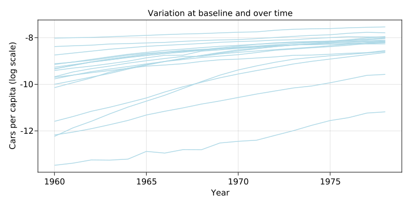
Below is an example of the number of cars per capita in certain countries over time using the gasoline dataset from the R package plm. Some noticeable facts about this dataset are 1) there is a clear difference in the number of cars between countries in the initial year of study (1960) 2) this initial difference is also far larger than the change within any one country over the time course of the study and 3) each country changes in a steady quite predictable fashion. The dataset contains other variables (income per capital and gas price) which may explain some of this variation in initial conditions and rate of change.
using CairoMakie, DataFrames, RDatasets, Statistics
df = dataset("plm", "Gasoline")
f = Figure(resolution = (800, 400))
ax = Axis(f[1,1], xlabel = "Year", ylabel = "Cars per capita (log scale)",
    title = "Variation at baseline and over time")
for country in unique(df.Country)
    msk = df.Country .== country
    lines!(ax,df.Year[msk],df.LCarPCap[msk],color = :lightblue)
end
f
Cars per capital for 18 countries (1960-1980)
What mixed effect models do is divide up the variation that exists in the data into several "buckets". At the highest level there is explained and unexplained variation. Explained variation is variation that is accounted for by your predictor features (covariates). These terms are often called fixed effects. For example, differences in blood pressure may be accounted for by differences in amount of salt intake or exercise quantity. Note that this can be both between and within units, two people may have different levels of average exercise quantity and one person may change their exercise quantity over time. Longitudinal data structures are very powerful in allowing us to examine difference in the effect of a variable both between and within units. For instance if we found that average exercise amount predicted a lowering in blood pressure but an individual increasing their exercise amount did not we might wonder whether 1) exercise was a proxy for something else or 2) does the change take a long time.
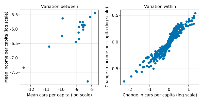
Looking again at the gasoline dataset, we can see that the number of cars per capita is higher in wealthier countries (the between country relationship), and also that as a country increases in wealth the number of cars per capita increases (the within country relationship). Indeed the within country relationship is quite clear and strong. In many cases (e.g. certain physiological signals) this relationship is often harder to discern due to the variation within units being of comparable size to "noise" factors such as measurement error and natural variation.
gdf = groupby(df,:Country)
mdf = combine(gdf, :LCarPCap => mean, :LIncomeP => mean)
df = leftjoin(df,mdf,on=:Country)
df.LIncomeP_change = df.LIncomeP - df.LIncomeP_mean
df.LCarPCap_change = df.LCarPCap - df.LCarPCap_mean
f = Figure(resolution = (800, 400))
ax1 = scatter(f[1, 1],mdf.LCarPCap_mean,mdf.LIncomeP_mean)
ax1.axis.xlabel = "Mean cars per capita (log scale)"
ax1.axis.ylabel = "Mean income per capita (log scale)"
ax1.axis.title = "Variation between"
ax2 = scatter(f[1, 2],df.LCarPCap_change,df.LIncomeP_change)
ax2.axis.xlabel = "Change in cars per capita (log scale)"
ax2.axis.ylabel = "Change in income per capita (log scale)"
ax2.axis.title = "Variation within"
f
Cars per capital and income per capita for 18 countries (1960-1980)
Unexplained variation is any variation that cannot be explained by values of (or variation in) the covariates. It is here that we really see the usefulness of mixed effect models. This unexplained variation is decomposed into the unexplained variation between units and within units. The between unit variation (the random effects) are the selling point of mixed effect models. Rather than associate with each term in our model (e.g. the intercept) a single fixed effect we might associate a distribution of effects. This distribution might have small or large degree of variation depending on the extent of the relevant unexplained variation that exists between our units. A notable fact is that we can have between unit variation in any term within our model, for instance the units might differ in their baseline values, suggesting random intercepts. They might also differ in the effect of a particular variable (e.g. time, effect of a drug) giving a random slope. A cartoon version of a random intercept and random slope situation is shown below.
A summary of the decomposition of variance view:
The descriptions above suggests you might only have one "level" of units. However, multilevel models can account for many levels of hierarchical clustering. For example, measurements within patients within medical practises.
Linear mixed effect models
The main practical issue with mixed effect models is while we may be able to write down a model that accounts for the variation we believe exists in the data (e.g. following some exploratory data analysis) fitting it turns out to be much harder than standard linear models. The remainder of this post demonstrates the estimation process for linear mixed effects models. With the notation \(x\) / \(X\) refering to a vector / matrix, and \(x_i\) / \(X_{ij}\) the element of a matrix / vector, a linear mixed effects model (LMM) can be written as
\[y = X\beta + Z b + \epsilon, b \sim N(0,\Lambda_{\theta}), \epsilon \sim N(0,\Sigma_{\theta})\]
where
\(\beta \in \mathcal{R}^p\) are the fixed effects, analogous to the coefficients in a standard linear model.
\(X \in \mathcal{R}^{Nn \times p}\) is the model matrix for the fixed effects containing the covariates / features.
The random vector \(b\) contains the random effects, with zero expected value and covariance matrix \(\Lambda_{\theta}\)
\(Z \in \mathcal{R}^{Nn \times n}\) is the model matrix for the random effects
\(\Sigma_{\theta}\) is the residual covariance matrix. It is often assumed that \(\Sigma_{\theta} = \sigma^2 I\)
\(\theta\) is the variance-covariance components, a vector of the random effect and residual variance parameters.
Motivating example
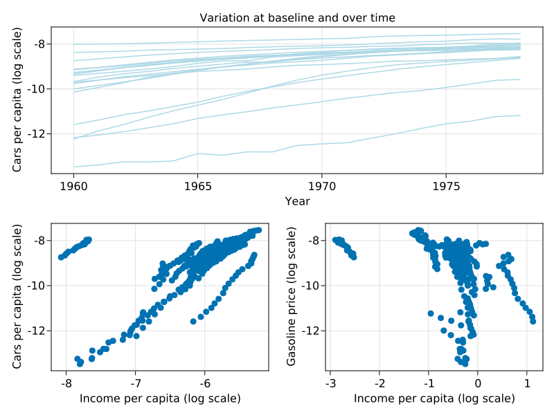
Using the gasoline dataset consider modelling car ownership (per capita) as a function of time (year), income (per capita) and gas price (inflation adjusted).
f = Figure(resolution = (800, 600))
ax = Axis(f[1,1:2], xlabel = "Year", ylabel = "Cars per capita (log scale)",
    title = "Variation at baseline and over time")
for country in unique(df.Country)
    msk = df.Country .== country
    lines!(ax,df.Year[msk],df.LCarPCap[msk],color = :lightblue)
end
ax1 = scatter(f[2, 1],df.LIncomeP,df.LCarPCap)
ax1.axis.ylabel = "Cars per capita (log scale)"
ax1.axis.xlabel = "Income per capita (log scale)"
ax2 = scatter(f[2, 2],df.LRPMG,df.LCarPCap)
ax2.axis.ylabel = "Gasoline price (log scale)"
ax2.axis.xlabel = "Income per capita (log scale)"
f
Cars per capital compared to several factors for 18 countries (1960-1980)
As mentioned above a commonly used form of the LMM is the random intercept model. In this situation for a single level (country over time) the resulting model for country \(i\) at time \(j\) is
I won't go into it's construction but it is worth thinking about what \(Z\) would look like in this case (if you run the code below you can print out \(Z\)), and how it would change it we added a time random effect. Doing this will give you a sense of how the size of \(Z\) can grow quite quickly while being a largely sparse matrix (filled with zeros).
Estimation
As mentioned LMMs are tricky to estimate, largely due to the presence of the unobserved random effects and additional need to decompose the outcome variance into several variance-covariance parameters. It is worth understanding the estimation process at least superficially as it can aid in debugging (commonly "why is my model taking so long to estimate!?") and understanding warning messages when using well tested packages written by others.
Theory
Feel free to skim this section. A common approach to estimation of LMMs is maximum likelihood estimation (MLE) or restricted MLE (REML) – but I'll just cover MLE here. As noted in Wood (2017) estimation of \(\beta\) and \(\theta\) could be based on the marginal distribution \(p(y)\) of the outcome
however this would involve the inversion of a \(Nn \times Nn\) matrix \(Z^t\Lambda_{\theta}Z + \Sigma_{\theta}\). As a result estimation is generally based on the the expression
\[p(y) = \int p(y,b) db = \int p(y|b)p(b) db\]
It is worth listing out some the log pdf of the distributions that are going to come up in the derivation of a the final expression. The log transform is taken to remove the exponents and convert multiplication into addition. Here and below \(c_x\) denotes a normalising constant for the distribution of \(x\).
Now we are ready to derive the estimation equations. Let \(\hat{b}\) be the MLE of \(p(y,b)\). Then utilising a Taylor expansion of \(p(y,b)\) about \(\hat{b}\) on the second line below we have
The term inside the integral can be recognised is an un-normalised Gaussian pdf with covariance \((Z^t\Sigma_{\theta}^{-1} Z + \Lambda_{\theta}^{-1})^{-1}\). The normalisation constant for this pdf would be \(\sqrt{|(Z^t\Sigma_{\theta}^{-1} Z + \Lambda_{\theta}^{-1})^{-1}| (2\pi)^{n}}\) and so, using the fact that \(|A^{-1}| = |A|^{-1}\) the result of the integral is
In practise we will work with the deviance (minus two times the log-likelihood), inputting our expressions for \(\text{log} p(y|b)\) and \(\text{log} p(b)\) from above gives the quantity to be minimised as
Notice that the random effects (e.g. the individual intercept or feature effect) are shrinkage estimates of what we would get if we let every unit have it's own intercept or feature effect, hence the term penalised least squares.
Then estimates of \(\theta\) can be based on the profile likelihood (deviance) \(d_p(\theta) = d(\hat{\beta},\theta)\).
Some other observations:
Several of the terms can be interpreted as a complexity penalties on the random effects or variance-covariance parameters.
A nicer approach is to let \(b = \Gamma_{\theta} u\) where \(u\) is a spherical normal variable (uncorrelated equal variance) and \(\Lambda_{\theta} = \Gamma_{\theta}^t\Gamma_{\theta}\), reducing the dimension of \(\theta\) by one (Bates et al, 2014).
Algorithm
How does estimation go in practise? Often a gradient free optimisation algorithm (Nelder-Mead or BOBYQA) is used for \(d_p\).
This is high level (but reasonable for understanding) view of how software packages like lme4 or MixedModel perform estimation for LMMs. See Bates et al (2015) for a detailed overview of the numerical linear algebra considerations in the implementations.
Julia implementation
For a more complete idea of how to code LMMs in practise see the source code for MixedModels.jl. The code below estimates \(\beta\) and the variance components \(\theta\).
## libraries
# linear algebra
using LinearAlgebra, SparseArrays
# optimisation
using Optim
import Statistics"""
Calculates log likelihood for LMM.
Internally calculates fixed and random effects given estimates of the variance-covariance components,
with modification of first three arguments βb, LL, rr. Designed for `lmm_fit`.Args
    βb  : vector of estimates of fixed and random effects
    D   : fixed and random effect design matrices
    DtD : D'D
    Dty : D'y
    y   : outcome vector
    logθ: log of variance-covariance components
    dim : tuple of dimensions"""
function loglik!(βb,D,DtD,Dty,y,logθ,dim)
    σ,σ_b = exp.(logθ)    # dimensions
    Nn,n,p = dim
    N = Nn/n    # estimation of \beta and b given theta
    diagf = diagm([repeat([0.0],p);repeat([1/σ_b^2],n)])
    LL = DtD ./ σ^2 + diagf
    βb[:] = LL \ (Dty ./ σ^2)    # -2 log likelihood (profile likelihood)
    logdetθ = logdet(DtD[(p+1):end,(p+1):end] ./ σ^2 + diagf[(p+1):end,(p+1):end])
    nll = (1/σ^2)*sum((y - D*βb).^2) + (1/σ_b^2)*sum(βb[(p+1):end].^2) + 2*logdetθ  + n*log(σ_b^2) + Nn*log(σ^2) + n*log(2*π)
    nll ./ 2
end"""
Estimate a LMMArgs
    X : Fixed effect design matrix
    Z : Random effect design matrix
    y : outcome
"""
function lmm_fit(X,Z,y)    # dimensions / data
    Nn = length(y)
    n = size(Z)[2]
    p = size(X)[2]
    dim = (Nn,n,p)
    D = [X Z]
    DtD = D'D
    Dty = D'y    # optimisation setup
    βb = zeros(n+p)
    θ0 = ones(2)    # optimise
    opt = optimize(var -> loglik!(βb,D,DtD,Dty,y,var,dim), log.(θ0), NelderMead())
    θ = exp.(Optim.minimizer(opt))    # output
    out = LMM(βb[1:p],θ,βb[(p+1):end],opt)
    out
end
"""
A struct to store the results of our LMM estimation
"""
struct LMM
    β
    θ
    b
    opt
end# A small test - the output should be approx [1.0,3.0]
N, n, p = 30, 100, 10
ids = repeat(1:n,inner=N)
X = [repeat([1.0],N*n) randn(N*n,p)]
β = randn(p+1)
θ2 = 3.0
b = sqrt(θ2) .* randn(n)
Z = sparse(kron(sparse(1I, n, n),repeat([1],N)))
y = X * β + Z * b + randn(N*n);
res = lmm_fit(X,Z,y);
println("Variance components: ",round.(res.θ .^ 2,digits=3))
Variance components: [1.06, 3.274]
Clearly it is still worth using MixedModels.jl but the benefit of being able to code it yourself is the freedom you get to make changes in the underlying algorithm and see the effects.
Example revisited
Estimating the car ownership model using lmm_fit gives the following results.
df.Time = df.Year .- 1965
n = length(unique(df.Country))
N = length(unique(df.Year))
X = [repeat([1.0],size(df)[1]) df.Time df.LIncomeP df.LRPMG]
Z = sparse(kron(sparse(1I, n, n),repeat([1],N)))
y = df.LCarPCap
res = lmm_fit(X,Z,y);
println("Variance components: ",round.(res.θ .^ 2,digits=3))
println("Fixed effects: ",round.(res.β,digits=4))
Estimating the car ownership model from above using MixedModels.jl gives the following results.
using MixedModels
m1 = fit(MixedModel, @formula(LCarPCap ~ 1 + Time + LIncomeP + LRPMG + (1|Country)), df)
println(m1)
Linear mixed model fit by maximum likelihood
 LCarPCap ~ 1 + Time + LIncomeP + LRPMG + (1 | Country)
   logLik   -2 logLik     AIC       AICc        BIC
    57.5230  -115.0460  -103.0460  -102.7952   -80.0371Variance components:
            Column   Variance Std.Dev.
Country  (Intercept)  1.627124 1.275588
Residual              0.028976 0.170223
 Number of obs: 342; levels of grouping factors: 18  Fixed-effects parameters:
────────────────────────────────────────────────────
                  Coef.  Std. Error      z  Pr(>|z|)
────────────────────────────────────────────────────
(Intercept)   6.69453    0.727785     9.20    <1e-19
Time         -0.0124492  0.00439073  -2.84    0.0046
LIncomeP      2.57169    0.104949    24.50    <1e-99
LRPMG        -0.195353   0.0807133   -2.42    0.0155
────────────────────────────────────────────────────
The results from the two approaches are similar, the minor differences can be attributed to use of different optimisation routines. Interpreting the results it looks like income is the most important factor in predicting increased car ownership. Gas prices decreasing and temporal trends are noiser seconds. Indeed the sign for time is negative which may be a result of some collinearity due to income and time increasing together. The intercept random effect still has reasonably large variation, although it is clearly smaller than what we would expect if time was the only covariate (see the first figure).
Conclusion
We've covered the background of why you might use mixed effects models, along with the estimation of linear mixed effects models. Some other interesting topics worth exploring are the estimation of generalised linear mixed effects models, and a comparison with taking a Bayesian approach to model estimation. Thanks for reading! :)
References
This document borrows from the following:
Wood, S. N. (2017). Generalized additive models: an introduction with R. CRC press.
Bates, D., Mächler, M., Bolker, B., & Walker, S. (2014). Fitting linear mixed-effects models using lme4. arXiv preprint arXiv:1406.5823.