minGPT in Julia using Flux!

By: Can Candan's Blog

Re-posted from: https://cancandan.github.io/julia/flux/machine-learning/2022/03/30/mingpt-julia.html

Introduction

As a learning exercise, I tried to port Andrey Karpathy’s awesome minGPT, which is based on Python and PyTorch to Julia and Flux. GPT is a language model, that is trained by the error signal of its prediction for the next element of a given sequence. Karpathy runs the model on three different problems, each in a distinct domain, but fitting this format; language, vision and math. Here I concentrate on the self contained math problem, in which we are interested in seeing whether the model can learn to do addition given two, two digit numbers. Therefore, we begin by creating a dataset where we encode the addition problem and its result as one string. The two, two digit numbers, and the result of addition, which is three digits (both inputs and the result padded with zeros if necessary), is encoded as a string. For example, the addition of 85 and 50 which results in 135 is encoded as the sequence [8, 5, 5, 0, 1, 3, 5]. Given 85 and 50, the model should predict 135. This amounts to predicting [8, 5, 5, 0, 1] given [8, 5, 5, 0]. Predicting [8, 5, 5, 0, 1, 3] given [8, 5, 5, 0, 1] and finally predicting [8, 5, 5, 0, 1, 3, 5] given [8, 5, 5, 0, 1, 3].

Hence, our input to the model will look like [8, 5, 5, 0, 1, 3]. For the ouput he considers a sequence like this [-100, -100, -100, 1, 3, 5]. The -100s are to be ignored here in the loss calculation. How this translates to Julia code can be understood from this part of the code:


Note that since the Julia indexing starts from 1, our labels start from 1, and we also have the -99. What I am doing is here is to one hot encode the digits and also the -100 (-99 in Julia) and drop that -99 in the last row (see that [1:end-1, :, :]) and then element wise multiply (the .* in the loss function). This amounts to ignoring known part of the given sequence in the loss calculation.

Components

It was quite straightforward to port all of the PyTorch components to Flux. For example below on the left you see the Python class definition for the CausalSelfAttention component, and on the right is how to define it in Julia.

Python

Julia

The meat of this component follows next. One thing that tripped me here, has been the application of the mask. As you can see, on the left below, the att variable is modified in-place by using the masked_fill function of PyTorch. Doing the same thing with Flux lead to an error saying Mutating arrays is not supported. I guess in-place modification is not possible in the current AD component of Flux, ie. Zygote. To work around that I added the upper triangular mask to the output att of the batch matrix multiplication operation, which I do using Flux functions batched_mul and batched_transpose. Note that here, Flux requires the batch dimesion to be the last, as evidenced by the difference in the order of B, T, C.

Python

Julia

Weight Decay and Optimiser

An interesting bit in Karpathy’s code is how he had to select the parameters of the model to apply weight decay to. The following lengthy function below is doing that:


In Flux one can implement the trainable function for this, as described in the docs. Getting inspiration from that, I added a decayed_trainable. In my custom optimiser code (that I adapted from the Flux’s ADAM) I handle the weight decay if the parameters needs to be decayed. Hence this is how I specify the parameters:


Flux docs mention the weight decayed version of ADAM, the ADAMW. But as far as I understand, this is not quite how Pytorch’s ADAMW works, so I grabbed the code of basic ADAM and added the bag of tricks Karpathy used in his code, like norm clipping the gradients and decoupled weight decay of selected parameters. To be precise I tried to implement the algorithm in the paper shown below, with these added bells and whistles.

ADAMW

Hence our optimiser looks like this:


Loss and Gradient Calculation

For training, we need a loss function and its gradient, computed on batches of data. So we get the ouput from the model, apply our cross entropy / softmax loss function via the Zygote.pullback to get both of these in one shot, and then hit to the optimiser Flux.Optimise.update! with it as shown:


Making it Fast

My model was training well at this point, but it was like 10x slower than the Python version, on the GPU. Having no idea what could possible make it run so slowly, I googled for Transformers in Julia, and of course found about Transformers.jl, a Julia library for Transformers. In this library, we see a custom implementation of the batched matrix multiplication AND how to efficiently differentiate it:


The batched_gemm! of the Transformers.jl lib shown above here is also hitting a CUDA version in the library. And indeed, bringing those in to my code, it started running as fast as Python. However, thanks to the wonderful people at Julia Slack (Michael Abbott, Andrew Dinhobl), I learned that all of this is already integrated into the Flux library. Hence no need to grab code from anywhere. Yay!.. For example, the efficient differentiation, is part of Flux now, in the form of a rrule of ChainRules.jl.


It turned out that, what made my code run extremely slowly was.. (wait for it).. NOT casting the output of the sqrt below to Float32. The function sqrt outputs here a Float64 and makes the whole chain afterwards VERY inefficient. So, number one thing to look out for when tracking down inefficiencies in Julia is making sure you are using the correct types.


Try it yourself

If you want to try this out yourself, this notebook shows what needs to be done, which I copy below for reference:

include("minGPT.jl")

using Random
Random.seed!(123)

ndigit=2

(trnx,trny),(tstx,tsty)=makeData(ndigit)    

map(addOneForJulia, [trnx, trny, tstx, tsty])

config = Dict("vocab_size"=>10, "n_embed"=>128, "attn_pdrop"=>0.1f0, "resid_pdrop"=>0.1f0, "embd_pdrop"=>0.1f0, "block_size"=>6, "n_layer"=>2, "n_head"=>4,
"max_epochs"=>110, "batch_size"=>512, "learning_rate"=>6f-4, "lr_decay"=>true, "warmup_tokens"=>1024, "final_tokens"=>50*size(trnx)[2]*(ndigit+1), "betas"=>(0.9f0, 0.95f0));

model = mytraining(trnx, trny, tstx, tsty, config)
Epoch: 1 Iter: 1 Train Loss: 2.95 lr_mult: 1.00 tokens: 1536
Epoch: 1 Iter: 11 Train Loss: 2.07 lr_mult: 1.00 tokens: 16896
Test Loss: 1.90209
Epoch: 2 Iter: 1 Train Loss: 1.98 lr_mult: 1.00 tokens: 25536
Epoch: 2 Iter: 11 Train Loss: 1.91 lr_mult: 1.00 tokens: 40896
Test Loss: 1.7956433
Epoch: 3 Iter: 1 Train Loss: 1.86 lr_mult: 1.00 tokens: 49536
Epoch: 3 Iter: 11 Train Loss: 1.78 lr_mult: 0.99 tokens: 64896
Test Loss: 1.7278897
Epoch: 4 Iter: 1 Train Loss: 1.76 lr_mult: 0.99 tokens: 73536
Epoch: 4 Iter: 11 Train Loss: 1.73 lr_mult: 0.99 tokens: 88896    
...    
Epoch: 109 Iter: 1 Train Loss: 0.01 lr_mult: 0.94 tokens: 2593536
Epoch: 109 Iter: 11 Train Loss: 0.00 lr_mult: 0.93 tokens: 2608896
Test Loss: 0.00010189927
Epoch: 110 Iter: 1 Train Loss: 0.01 lr_mult: 0.92 tokens: 2617536
Epoch: 110 Iter: 11 Train Loss: 0.01 lr_mult: 0.91 tokens: 2632896
Test Loss: 0.0002310586
give_exam(model, trnx, trny, config)
tot: 8000 tot_correct: 7999
give_exam(model, tstx, tsty, config)
tot: 2000 tot_correct: 2000
Life expectancy and transition in cause of death patterns

By: Karl Pettersson

Re-posted from: https://www.dusty-test.klpn.se/posts/2022-03-27-transition.html

Life expectancy and transition in cause of death patterns

Posted on 2022-03-27

by Karl Pettersson.

Tags: ,

This week, the Swedish statistical agency has published life tables for
Sweden 2021 (Statistics Sweden 2023). With the first waves of the COVID pandemic, life
expectancy at birth decreased from 84.73 years for females and 81.34
years for males in 2019 to 84.29/80.60 years in 2020. For 2021, the
numbers were again 84.82/81.21 years. This reflects, of course, the
decreased COVID mortality due to vaccination. Moreover, the flu A(H3N2)
wave, which peaked around Christmas with rather high rates of illness
among young people, did not cause substantial excess mortality, which
may, in part, be due to people with respiratory symptoms having less
contacts than usual with older people and other risk groups.

The increase in life expectancy in Sweden, and many other countries, up
until the mid-20th century was largely driven by decreasing childhood
mortality, which also caused changes in the cause of death patterns,
with directly communicable diseases becoming less common relative to
age-related diseases, such as circulatory diseases and cancer. In
contrast, the continued increase in rich countries after that, which was
temporarily interrupted by the pandemic, is largely due to decreased
mortality at older ages.

Vishnevsky (2017) discusses the development in life expectancy and causes
of death after 1960 in Russia, compared to high-income countries, in
particular Western European countries. In the EU-15 countries,
age-standardised mortality rates from circulatory, external and
respiratory causes have decreased greatly since 1970, while cancer
mortality has decreased modestly. The proportion of deaths from
circulatory causes has also decreased (from nearly 50 percent to about
30 percent), while the proportion of deaths from cancer has increased
(from about 20 percent to about 30 percent). No such changes have
occurred in Russia, where life expectancy has not improved much since
the 1960s (although it has improved relative to the dramatic increases
in mortality during the 1990s).

From this, one might conclude that the increased life expectancy in rich
countries largely has been about decreased circulatory mortality.
However, Vishnevsky points out that focusing on standardised rates for
all ages hides a significant increase in life expectancy for those dying
also of non-circulatory causes. In Sweden, for example, the life
expectancy for people dying of cancer or other neoplasms increased 8.2
years for females and 7.6 years for males during to period 1960–2010.
The corresponding increase for circulatory diseases (where life
expectancy was higher than for cancer already in 1960) is 8.0/6.8 years.
It is clear that this reflects a marked decrease in cancer mortality at
young ages, a point similar to what has been made earlier by researchers
like Riggs (1994).

One factor not discussed by Vishnevsky is the impact of changing
practices in reporting causes of death over a long time. For example,
the increase in life expectancy has been particularly strong for the
residual category, other diseases, in Sweden, with 20.0 years for
females and 17.8 years for males. This category includes dementia, which
was a rare underlying cause of death in 1960. Back then, most people
with dementia probably had circulatory or respiratory causes reported
instead, and the other category was dominated by other causes, with a
much lower life expectancy.

In light of this, it may be interesting to compare the correlation
between general life expectancy and proportion of deaths ascribed to
different causes in varying countries more in detail. I made a Julia
package, MortIntl, which can be
used to analyse such trends, based on cause-specific mortality data from
WHO (2025) and life tables from University of California, Berkeley and Max Planck Institute for Demographic Research (2022). It uses a configuration similar to
my earlier Mortchartgen,
which I have used to generate Mortality
Charts
, but extracts data directly from
the data files using AWK instead of relying on a SQL database.

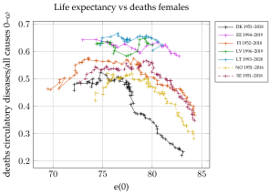
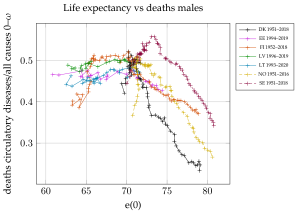
Fig. 1 and fig. 2 show female and male life expectancy at birth in
relation to proportion of deaths from circulatory causes (as defined for
Mortality Charts) for
the Nordic and Baltic countries, with Iceland excluded due to small
population.1

Figure 1: Circulatory deaths vs life expectancy females Nordic and Baltic countries.
Figure 2: Circulatory deaths vs life expectancy males Nordic and Baltic countries.

The charts clearly show that improvements in life expectancy continued
for a long time among, for example, females in Finland and Sweden, after
circulatory causes became dominant, without any substantial change in
the proportion of deaths ascribed to these causes. That proportion
really started decreasing after the 1980s, when dementia became more
commonly reported (see Mortality
Charts
).

The Baltic countries, especially Estonia, have in recent years attained
a female life expectancy close to the Nordic countries, but the
proportion of circulatory deaths there is higher than it has been in the
Nordic countries at any point in time. In contrast, Denmark, has had a
lower proportion of circulatory deaths than the other Nordic countries,
a pattern which has been more pronounced in recent decades. The
difference in circulatory deaths between Denmark and Estonia in recent
years, when both have had similar life expectancy among females, is
greater than the temporal variation, over nearly 70 years, in any of the
Nordic countries.

From this, it seems that clear that great caution is warranted in
drawing any epidemiological conclusions from trends for officially
reported circulatory mortality over all ages.

References

Riggs, J. E. 1994. “The cohort mortality perspective: The emperor′s new clothes of epidemiology, an illustration using cancer mortality.” Regulatory Toxicology and Pharmacology 19 (2): 202–210. doi:10.1006/rtph.1994.1018.
Statistics Sweden. 2023. “Life table by sex and age.” https://www.statistikdatabasen.scb.se/goto/en/ssd/LivslangdEttariga.
University of California, Berkeley and Max Planck Institute for Demographic Research. 2022. Human Mortality Database.” https://www.mortality.org.
Vishnevsky, Anatoly. 2017. “Mortality in russia: The second epidemiological revolution that never was.” Demographic Review 2 (5): 4–33. doi:10.17323/demreview.v2i5.5581.
WHO. 2025. “WHO Mortality Database.” https://www.who.int/data/data-collection-tools/who-mortality-database.

  1. The charts can be generated by cloning the blog
    repository
    , installing
    MortIntl with the relevant data files, as described in the
    documentation, and running circall_e0_baltnord.jl in the
    subdirectory postdata/2022-03-27-transition.↩︎

Life expectancy and transition in cause of death patterns

By: Karl Pettersson

Re-posted from: https://static-dust.klpn.se/posts/2022-03-27-transition.html

Life expectancy and transition in cause of death patterns

Posted on 2022-03-27

by Karl Pettersson.

Tags: epidemiology, julia

This week, the Swedish statistical agency has published life tables for
Sweden 2021 (Statistics Sweden 2022). With the first waves of the COVID pandemic, life
expectancy at birth decreased from 84.73 years for females and 81.34
years for males in 2019 to 84.29/80.60 years in 2020. For 2021, the
numbers were again 84.82/81.21 years. This reflects, of course, the
decreased COVID mortality due to vaccination. Moreover, the flu A(H3N2)
wave, which peaked around Christmas with rather high rates of illness
among young people, did not cause substantial excess mortality, which
may, in part, be due to people with respiratory symptoms having less
contacts than usual with older people and other risk groups.

The increase in life expectancy in Sweden, and many other countries, up
until the mid-20th century was largely driven by decreasing childhood
mortality, which also caused changes in the cause of death patterns,
with directly communicable diseases becoming less common relative to
age-related diseases, such as circulatory diseases and cancer. In
contrast, the continued increase in rich countries after that, which was
temporarily interrupted by the pandemic, is largely due to decreased
mortality at older ages.

Vishnevsky (2017) discusses the development in life expectancy and causes
of death after 1960 in Russia, compared to high-income countries, in
particular Western European countries. In the EU-15 countries,
age-standardised mortality rates from circulatory, external and
respiratory causes have decreased greatly since 1970, while cancer
mortality has decreased modestly. The proportion of deaths from
circulatory causes has also decreased (from nearly 50 percent to about
30 percent), while the proportion of deaths from cancer has increased
(from about 20 percent to about 30 percent). No such changes have
occurred in Russia, where life expectancy has not improved much since
the 1960s (although it has improved relative to the dramatic increases
in mortality during the 1990s).

From this, one might conclude that the increased life expectancy in rich
countries largely has been about decreased circulatory mortality.
However, Vishnevsky points out that focusing on standardised rates for
all ages hides a significant increase in life expectancy for those dying
also of non-circulatory causes. In Sweden, for example, the life
expectancy for people dying of cancer or other neoplasms increased 8.2
years for females and 7.6 years for males during to period 1960–2010.
The corresponding increase for circulatory diseases (where life
expectancy was higher than for cancer already in 1960) is 8.0/6.8 years.
It is clear that this reflects a marked decrease in cancer mortality at
young ages, a point similar to what has been made earlier by researchers
like Riggs (1994).

One factor not discussed by Vishnevsky is the impact of changing
practices in reporting causes of death over a long time. For example,
the increase in life expectancy has been particularly strong for the
residual category, other diseases, in Sweden, with 20.0 years for
females and 17.8 years for males. This category includes dementia, which
was a rare underlying cause of death in 1960. Back then, most people
with dementia probably had circulatory or respiratory causes reported
instead, and the other category was dominated by other causes, with a
much lower life expectancy.

In light of this, it may be interesting to compare the correlation
between general life expectancy and proportion of deaths ascribed to
different causes in varying countries more in detail. I made a Julia
package, MortIntl, which can be
used to analyse such trends, based on cause-specific mortality data from
WHO (2022) and life tables from University of California, Berkeley and Max Planck Institute for Demographic Research (2022). It uses a configuration similar to
my earlier Mortchartgen,
which I have used to generate Mortality
Charts
, but extracts data directly from
the data files using AWK instead of relying on a SQL database.

Fig. 1 and fig. 2 show female and male life expectancy at birth in
relation to proportion of deaths from circulatory causes (as defined for
Mortality Charts) for
the Nordic and Baltic countries, with Iceland excluded due to small
population.1

Figure 1: Circulatory deaths vs life expectancy females Nordic and Baltic countries.
Figure 2: Circulatory deaths vs life expectancy males Nordic and Baltic countries.

The charts clearly show that improvements in life expectancy continued
for a long time among, for example, females in Finland and Sweden, after
circulatory causes became dominant, without any substantial change in
the proportion of deaths ascribed to these causes. That proportion
really started decreasing after the 1980s, when dementia became more
commonly reported (see Mortality
Charts
).

The Baltic countries, especially Estonia, have in recent years attained
a female life expectancy close to the Nordic countries, but the
proportion of circulatory deaths there is higher than it has been in the
Nordic countries at any point in time. In contrast, Denmark, has had a
lower proportion of circulatory deaths than the other Nordic countries,
a pattern which has been more pronounced in recent decades. The
difference in circulatory deaths between Denmark and Estonia in recent
years, when both have had similar life expectancy among females, is
greater than the temporal variation, over nearly 70 years, in any of the
Nordic countries.

From this, it seems that clear that great caution is warranted in
drawing any epidemiological conclusions from trends for officially
reported circulatory mortality over all ages.

References

Riggs, J. E. 1994. “The cohort mortality perspective: The emperor′s new clothes of epidemiology, an illustration using cancer mortality.” Regulatory Toxicology and Pharmacology 19 (2): 202–210. doi:10.1006/rtph.1994.1018.
Statistics Sweden. 2022. “Life table by sex and age.” https://www.statistikdatabasen.scb.se/goto/en/ssd/LivslangdEttariga.
University of California, Berkeley and Max Planck Institute for Demographic Research. 2022. “Coronavirus (COVID-19) infection survey, UK: 7 january 2022.” https://www.mortality.org.
Vishnevsky, Anatoly. 2017. “Mortality in russia: The second epidemiological revolution that never was.” Demographic Review 2 (5): 4–33. doi:10.17323/demreview.v2i5.5581.
WHO. 2022. “WHO Mortality Database.” https://www.who.int/data/data-collection-tools/who-mortality-database.

  1. The charts can be generated by cloning the blog
    repository
    , installing
    MortIntl with the relevant data files, as described in the
    documentation, and running circall_e0_baltnord.jl in the
    subdirectory postdata/2022-03-27-transition.↩︎