By: Julia on μβ

Re-posted from: https://matbesancon.xyz/post/2022-04-29-expression-trees/

Today was the release of SCIP.jl v0.11, the first release switching to SCIP 8.
The major change in this (massive) release was the rewrite of the nonlinear optimization part, using a so-called expression framework.
The rewrite of the wrapper had some fairly tedious parts, debugging C shared libraries is quickly a mess with cryptic error messages.
But the nonlinear rewrite gave me the opportunity to tweak the way Julia expressions are passed to SCIP in a minor way.

Table of Contents

SCIP expressions

I will not go in depth into the new expression framework and will instead reference these slides
but more importantly the SCIP 8 release report

The key part is that in a nonlinear expression, each operand is defined as an expression handler, and new ones can be introduced by users.
Several specialized constraint types or constraint handlers in SCIP terminology were also removed, using the expression framework with
a generic nonlinear constraint instead.

The Julia wrapper initial framework

As a Lisp-inspired language, (some would even a Lisp dialect),
Julia is a homoiconic language: valid Julia code can always be represented and stored in a primitive data structure.
In this case, the tree-like structure is Expr with fields head and args:

julia> expr = :(3 + 1/x)
:(3 + 1 / x)

julia> expr.head
:call

julia> expr.args
3-element Vector{Any}:
  :+
 3
  :(1 / x)

The SCIP.jl wrapper recursively destructures the Julia expression and builds up corresponding SCIP
expressions, a SCIP data structure defined either as a leaf (a simple value or a variable)
or as an operand and a number of subexpressions.
This is done through a push_expr! function which either:

• Creates and returns a single variable expression if the expression is a variable
• Creates and returns a single value expression if the expression is a constant
• If the expression is a function f(arg1, arg2...), calls push_expr! on all arguments, and then creates and returns the SCIP expression corresponding to f.

One part remains problematic, imagine an expression like 3 * exp(x) + 0.5 * f(4.3), where f
is not a primitive supported by SCIP. It should not have to be indeed, because that part of the expression
could be evaluated at expression compile-time. But if one is walking down the expression sub-parts,
there was no way to know that a given part is a pure value, the expression-constructing procedure would
first create a SCIP expression for 4.3 and then try to find a function for f to apply with this expression
pointer as argument. This was the use case initially reported in this issue
at a time when SCIP did not support trigonometric functions yet.

Another motivation for solving this issue is on the computational and memory burden.
Imagine your expression is now 3 * exp(x) + 0.1 * cos(0.1) + 0.2 * cos(0.2) + ... + 100.0 * cos(100.0).
This will require producing 2 * 1000 expressions for a constant, declared, allocated and passed down to SCIP.
The solver will then likely preprocess all constant expressions to reduce them down, so it ends up being a lot of
work done on one end to undo immediately on the other.

A lazified expression declaration

Make push_expr! return two values (scip_expr, pure_value), with the second being a Boolean for whether the expression is a pure value or not.
At any leaf computing f(arg1, arg2...).

If the expression of all arguments are pure_value, do not compute the expression and just return a null pointer, pure_value is true for this expression.

If at least one of the arguments is not a pure_value, we need to compute the actual expression. None of the pure_value arguments were declared as SCIP expressions yet, we create a leaf value expression for them with Meta.eval(arg_i). The non-pure value arguments already have a correct corresponding SCIP expression pointer. pure_value is false for this expression.

Note here that we are traversing some sub-expressions twice, once when walking down the tree and once more hidden with Meta.eval(arg_i) which computes the value for said expression, where we delegate the expression value computation to Julia. An alternative would be to return a triplet from every push_expr! call (expr_pointer, pure_value, val) and evaluate at
each pure_value node the value of f(args...), with the value of the arguments already computed. This would however complexity the code in the wrapper with no advantage of the runtime,
the expression evaluation is not a bottleneck for expressions that can realistically be tackled by a global optimization solver like SCIP.

By: Dean Markwick's Blog -- Julia

Re-posted from: https://dm13450.github.io/2022/04/28/Volatility-methods.html

Volatility measures the scales of price changes and is an easy way to
describe how busy markets are. High volatility means there are periods
of large price changes and vice versa, low volatility means periods of
small changes. In this post, I’ll show you how to measure realised
volatility and demonstrate how it can be used. If you just want a live
view of crypto volatility, take a look at
cryptoliquiditymetrics where I have added in a new card with the volatility over the last 24 hours.

Enjoy these types of posts? Then you should sign up for my newsletter. It’s a short monthly recap of anything and everything I’ve found interesting recently plus
any posts I’ve written. So sign up and stay informed!

To start with we will be looking at daily data. Using my
CoinbasePro.jl package in a Julia we can get the last 300 days OHLC
prices.

I’m running Julia 1.7 and all the packages were updated using
Pkg.update() at the time of this post.

using CoinbasePro
using Dates
using Plots, StatsPlots
using DataFrames, DataFramesMeta
using RollingFunctions

From my CoinbasePro.jl
package, we can pull in the daily candles of Bitcoin. 86400 is the
frequency for daily data. Coinbase restrict you to just 300 data
points

dailydata = CoinbasePro.candles("BTC-USD", now()-Day(300), now(), 86400);
sort!(dailydata, :time)
dailydata = @transform(dailydata, :time = Date.(:time))
first(dailydata, 4)

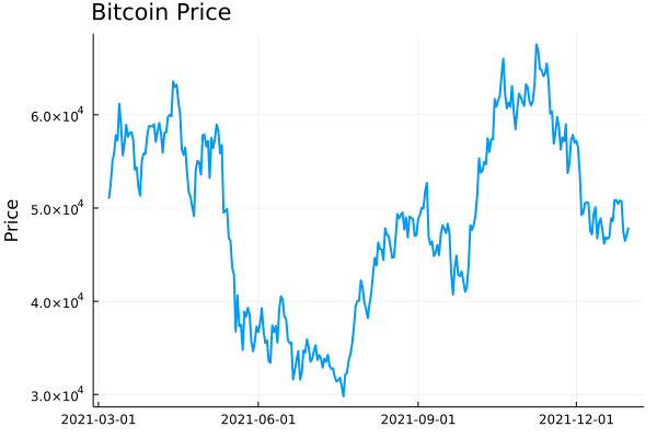
Plotting this gives you the typical price path. Now realised
volatility is a measure of how varied this price was
over time. Was it stable or were there wild swings?

plot(dailydata.time, dailydata.close, label = :none, 
     ylabel = "Price", title = "Bitcoin Price", titleloc = :left, linewidth = 2)

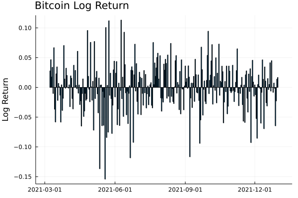
To calculate this variation, we need to add in the log-returns.

dailydata = @transform(dailydata, :returns = [NaN; diff(log.(:close))]);
bar(dailydata.time[2:end], dailydata.returns[2:end], 
    label=:none, 
    ylabel = "Log Return", title = "Bitcoin Log Return", titleloc = :left)

We can start by looking at this from a distribution perspective. If we
assume the log-returns (\(r\)) are from a normal distribution, with
zero mean, the standard deviation of this distribution is the equivalent to the
volatility

\[r \sim N(0, \sigma ^2),\]

so \(\sigma\) is how we will refer to volatility. From this, you can
see how high volatility leads to wide variations in prices. Each
log-return sample has a wider range of values that it could be.

So by taking the running standard deviation of the log-returns we can
estimate the volatility and how it changes over time. Using the RollingFunctions.jl package this is a one-liner.

dailydata = @transform(dailydata, :volatility = runstd(:returns, 30))
plot(dailydata.time, dailydata.volatility, title = "Bitcoin Volatility", titleloc = :left, label=:none, linewidth = 2)

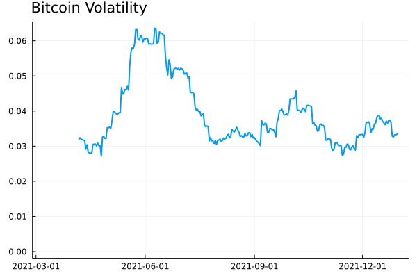
There was high volatility over June this year as the price of Bitcoin
crashed. It’s been fairly stable since then, hovering around 0.03
and 0.04. How does this compare though to the S&P 500 as a general
indicator of the stop market? We know Bitcoin is more volatile than
the stock market, but how much more?

I’ll load up the AlphaVantage.jl package to pull the daily prices of
the SPY ETF and repeat the calculation; adding the log-returns and
taking the rolling standard deviation.

using AlphaVantage, CSV

stockPrices = AlphaVantage.time_series_daily("SPY", datatype="csv", outputsize="full", parser = x -> CSV.File(IOBuffer(x.body))) |> DataFrame
sort!(stockPrices, :timestamp)
stockPrices = @subset(stockPrices, :timestamp .>= minimum(dailydata.time));

Again, add in the log-returns and calculate the rolling standard
deviation to estimate the volatility.

stockPrices = @transform(stockPrices, :returns = [NaN; diff(log.(:close))])
stockPrices = @transform(stockPrices, :volatility = runstd(:returns, 30));

volPlot = plot(dailydata.time, dailydata.volatility, label="BTC", 
               ylabel = "Volatility", title = "Volatility", titleloc = :left, linewidth = 2)
volPlot = plot!(volPlot, stockPrices.timestamp, stockPrices.volatility, label = "SPY", linewidth = 2)

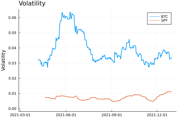
As expected, Bitcoin volatility is much higher. Let’s take the log of
the volatility to look zoom in on the detail.

volPlot = plot(dailydata.time, log.(dailydata.volatility), 
               label="BTC", ylabel = "Log Volatility", title = "Log Volatility", 
               titleloc = :left, linewidth = 2)
volPlot = plot!(volPlot, stockPrices.timestamp, log.(stockPrices.volatility), label = "SPY", linewidth = 2)

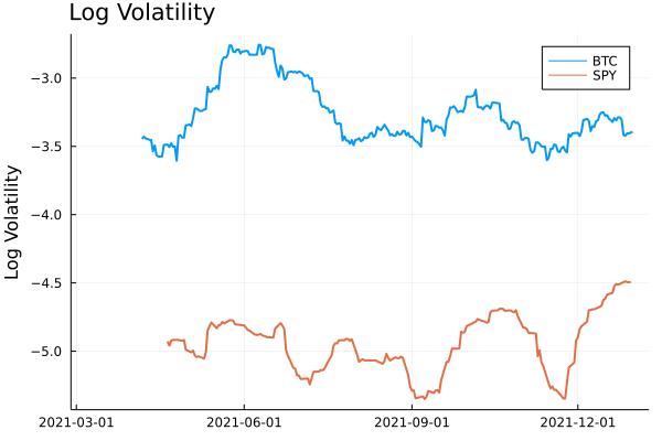
Interestingly the SPY has had a resurgence in volatility as we move
towards the end of the year. One thing to point out though is the
slight difference in look back periods for the two products. Bitcoin
does not observe weekends or holidays, so 30 rows previously are
always 30 days, but for SPY this is the case as there are weekends and
trading holidays. In this illustrative example, it isn’t too much of an
issue, but if you were to take it further and perhaps look at the
correlation between the volatilities, this is something you would need
to account for.

A Higher Frequency Volatility

So far it has all been on daily observations, your classic dataset to
practise on. But I am always banging on about high-frequency finance,
so let’s look at more frequent data and understand how the volatility
looks at finer timescales.

This time we will pull the 5-minute candle bar data of both Bitcoin
and SPY and repeat the calculation.

1. Calculate the log-returns of the close to close bars
2. Calculate the rolling standard deviation by looking back 20 rows.

minuteData_spy = AlphaVantage.time_series_intraday_extended("SPY", "5min", "year1month1", parser = x -> CSV.File(IOBuffer(x.body))) |> DataFrame
minuteData_spy = @transform(minuteData_spy, :time = DateTime.(:time, dateformat"yyyy-mm-dd HH:MM:SS"))
minuteData_btc = CoinbasePro.candles("BTC-USD", maximum(minuteData_spy.time)-Day(1), maximum(minuteData_spy.time),300);

combData = leftjoin(minuteData_spy[!, [:time, :close]], minuteData_btc[!, [:time, :close]], on=[:time], makeunique=true)
rename!(combData, ["time", "spy", "btc"])
combData = combData[2:end, :]
dropmissing!(combData)
sort!(combData, :time)
first(combData, 3)

For 5 minute data, we will use a look-back period of 20 rows, which gives us 100 minutes, so a little under 2 hours.

combData = @transform(combData, :spy_returns = [NaN; diff(log.(:spy))],
                                :btc_returns = [NaN; diff(log.(:btc))])
combData = @transform(combData, :spy_vol = runstd(:spy_returns, 20),
                                :btc_vol = runstd(:btc_returns, 20))
combData = combData[2:end, :];

Plotting it all again!

vol_tks = minimum(combData.time):Hour(6):maximum(combData.time)
vol_tkslbl = Dates.format.(vol_tks, "e HH:MM")

returnPlot = plot(combData.time[2:end], cumsum(combData.btc_returns[2:end]), 
                  label="BTC", title = "Cumulative Returns", xticks = (vol_tks, vol_tkslbl),
                  linewidth = 2, legend=:topleft)
returnPlot = plot!(returnPlot, combData.time[2:end], cumsum(combData.spy_returns[2:end]), label="SPY",
                   xticks = (vol_tks, vol_tkslbl),
                   linewidth = 2)


volPlot = plot(combData.time, combData.btc_vol * sqrt(24 * 20), 
    label="BTC", xticks = (vol_tks, vol_tkslbl), titleloc = :left, linewidth = 2)
volPlot = plot!(combData.time, combData.spy_vol * sqrt(24 * 20), label="SPY", title = "Volatility",
               xticks = (vol_tks, vol_tkslbl), titleloc = :left, linewidth = 2)

plot(returnPlot, volPlot)

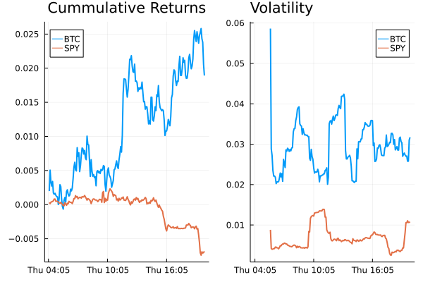
On the left-hand side, we have the cumulative return of the two
assets on the 30th of December, and on the right the corresponding
volatility. Bitcoin still has higher volatility whereas SPY has been
relatively stable with just some jumps.

Simplifying the Calculation

Rolling the standard deviation isn’t the efficient way of calculating the volatility and can also be simplified down to a more efficient calculation.

The standard deviation is defined as:

\[\sigma ^2 = \mathbb{E} (r^2) + \mathbb{E} (r) ^2\]

if we assume there is no trend in the returns so that the average is zero:

\[\mathbb{E} (r) = 0\]

then we get just the first term

\[\sigma ^2 = \frac{1}{N} \sum _{i=1} ^N r^2\]

which is simply proportional to the sum of squares. Hence why you will
hear that the realised variance is referred to as the sum of squares.

Once again, let’s pull the data and repeat the previous calculations
but this time adding another column that is the rolling summation of
the square of the returns.

minutedata = CoinbasePro.candles("BTC-USD", now()-Day(1) - Hour(1), now(), 5*60)
sort!(minutedata, :time)
minutedata = @transform(minutedata, :close_close_return = [NaN; diff(log.(:close))])
minutedata = minutedata[2:end, :]
first(minutedata, 4)

minutedata = @transform(minutedata,
                                    :new_vol_5 = running(sum, :close_close_return .^2, 20),
                                    :vol_5 = runstd(:close_close_return, 20))
minutedata = minutedata[2:end, :]
minutedata[1:5, [:time, :new_vol_5, :vol_5]]

vol_tks = minimum(minutedata.time):Hour(8):maximum(minutedata.time)
vol_tkslbl = Dates.format.(vol_tks, "e HH:MM")

ss_vol = plot(minutedata.time, sqrt.(288 * minutedata.new_vol_5), titleloc = :left, 
              title = "Sum of Squares", label=:none, xticks = (vol_tks, vol_tkslbl), linewidth = 2)
std_vol = plot(minutedata.time, sqrt.(288 * minutedata.vol_5), titleloc = :left, 
               title = "Standard Deviation", label=:none, xticks = (vol_tks, vol_tkslbl), linewidth = 2)
plot(ss_vol, std_vol)

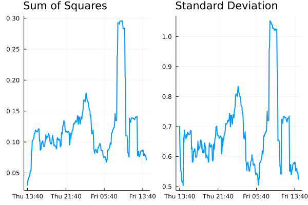
Both methods show represent the relative changes equally. There are
some notable edge effects in the standard deviation method, but
overall, our assumptions look fine. The y-scales are different though
as there are some constant factor differences between the two methods.

Comparing Crypto Volatilities

Let’s see how the volatility changes across some different
currencies. We define a function that calculates the close to close
return and iterate through some different currencies.

function calc_vol(ccy)
    minutedata = CoinbasePro.candles(ccy, now()-Day(1) - Hour(1), now(), 5*60)
    sort!(minutedata, :time)
    minutedata = @transform(minutedata, :close_close_return = [NaN; diff(log.(:close))])
    minutedata = minutedata[2:end, :]
    minutedata = @transform(minutedata, :var = 288*running(sum, :close_close_return .^2, 20))
    minutedata
    minutedata[21:end, :]
end

Let’s choose the classics BTC and ETH, the meme that is SHIB and
finally EURUSD (the crypto version).

p = plot(legend=:topleft, ylabel = "Realised Volatility")
for ccy in ["BTC-USD", "ETH-USD", "USDC-EUR", "SHIB-USD"]
    voldata = calc_vol(ccy)
    vol_tks = minimum(voldata.time):Hour(4):maximum(voldata.time)
    vol_tkslbl = Dates.format.(vol_tks, "e HH:MM")
    plot!(voldata.time, sqrt.(voldata.var), label = ccy, 
          xticks = (vol_tks, vol_tkslbl), linewidth = 2)
end
p

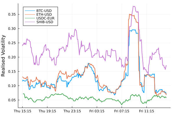
SHIB has higher overall volatility. ETH and BTC have very comparable
volatilities moving together. EURUSD has the lowest overall (as we
would expect), but interesting to see how it moved higher just as the
cryptos did at about 9 am.

An Update to CryptoLiquidityMetrics

So I’ve taken everything we’ve learnt here and implemented it into
cryptoliquiditymetrics.com. It is a new panel (bottom right) and
calculated all through Javascript.

How does this help you?

Knowing the volatility helps you get an idea of how easy it is to trade
or what strategy to use. When volatility is high and the price is
moving about it might be better to be more aggressive and make sure your trade
happens. Whereas if it is a stable market without too much volatility
you could be more passive and just wait, trading slowly and picking
good prices.

Just another addition to my Javascript side project!