By: Tamás K. Papp

Re-posted from: https://tamaspapp.eu/pages/blog/2022/hermite-approximation-spectralkit/index.html

When simulating from an economic model, I had to approximate a function \(f(x; \theta): [0,1] \to [0,1]\) for a variety of \(\theta\)s. \(f\) itself has to be solved for numerically, but otherwise it is pretty friendly, being continuous and increasing, with \(f(0)=0\) and \(f(1)=1\).

After profiling, this turned out to be the most costly part, so I had to approximate it. Since I needed derivatives \(f'(x)\), I was wondering whether making the approximation match them (known as a Hermite interpolation) would increase accuracy.

The (pedagogical, unoptimized) code below sums up the gist of my numerical experiments, with f below standing in for my implicitly solved function. It also demonstrates the new features of SpectralKit.jl v0.10.

First, we set up the problem:

using SpectralKit, PGFPlotsX, DisplayAsf(x) = (exp(x) - 1) / (exp(1) - 1)
f′(x) = exp(x) / (exp(1) - 1)
const I = BoundedLinear(0, 1)   # interval we map from

Then define an interpolation using N Chebyshev nodes, matching the values.

function interpolation0(f, N)
    basis = Chebyshev(EndpointGrid(), N)
    ϕ = collocation_matrix(basis) \ map(f ∘ from_pm1(I), grid(basis))
    linear_combination(basis, ϕ) ∘ to_pm1(I)
end;

Same exercise, but with the derivatives too, so we need two bases, one with double the number of functions (so we need to make sure N is even), while we just use N/2 for the nodes.

function interpolation01(f, f′, N)
    @assert iseven(N)
    basis1 = Chebyshev(EndpointGrid(), N ÷ 2) # nodes from this one
    basis2 = Chebyshev(EndpointGrid(), N)     # evaluate on this basis
    x = from_pm1.(I, grid(basis1))            # map nodes from [-1,1]
    M = collocation_matrix(basis2, to_pm1.(I, derivatives.(x)))
    ϕ = vcat(map(y -> y[0], M), map(y -> y[1], M)) \ vcat(f.(x), f′.(x))
    linear_combination(basis2, ϕ) ∘ to_pm1(I)
end;

Importantly, note that mapping to [-1,1] for the collocation matrix has to be preceded by lifting to derivatives.

Then calculate the max abs difference, in digits (log10).

function log10_max_abs_diff(f, f̂; M = 1000)
    x = range(0, 1; length = M)
    log10(maximum(@. abs(f(x) - f̂(x))))
end;

Then let's explore the errors in values …

Ns = 4:2:20
errors = [(log10_max_abs_diff(f, interpolation0(f, N)),
           log10_max_abs_diff(f, interpolation01(f, f′, N)))
          for N in Ns]

9-element Vector{Tuple{Float64, Float64}}:
 (-3.1996028783051695, -2.594513489315976)
 (-5.882145733021446, -5.488666848393999)
 (-8.835160643191552, -8.232779398084544)
 (-11.994023867372805, -11.44897859894945)
 (-15.176438519807359, -14.664555158828485)
 (-15.35252977886304, -15.35252977886304)
 (-15.255619765854984, -15.35252977886304)
 (-15.35252977886304, -15.35252977886304)
 (-15.35252977886304, -15.35252977886304)

… and derivatives.

d_errors = [(log10_max_abs_diff(f′, (x -> x[1]) ∘ interpolation0(f, N) ∘ derivatives),
             log10_max_abs_diff(f′, (x -> x[1]) ∘ interpolation01(f, f′, N) ∘ derivatives))
            for N in Ns]

9-element Vector{Tuple{Float64, Float64}}:
 (-2.0758500387125216, -2.093336352131656)
 (-4.549339116162139, -4.611253272379436)
 (-7.363367596306161, -7.429305371299876)
 (-10.417554370684012, -10.485171320264207)
 (-13.381718167990524, -13.689771947181466)
 (-13.834015838985154, -14.374806173574193)
 (-14.03551167781493, -14.539616422220185)
 (-13.724140848812729, -14.750469787535078)
 (-13.714040521908403, -14.724140848812729)

Finally the plots:

@pgf Axis({ xlabel = "number of basis functions",
            ylabel = "log10 abs error in values",
            legend_cell_align= "left" },
          PlotInc(Table(Ns, first.(errors))),
          LegendEntry("fitting values"),
          PlotInc(Table(Ns, last.(errors))),
          LegendEntry("fitting values and derivatives")) |> DisplayAs.SVG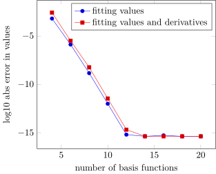

@pgf Axis({ xlabel = "number of basis functions",
            ylabel = "log10 abs error in values",
            legend_cell_align= "left" },
          PlotInc(Table(Ns, first.(d_errors))),
          LegendEntry("fitting values"),
          PlotInc(Table(Ns, last.(d_errors))),
          LegendEntry("fitting values and derivatives")) |> DisplayAs.SVG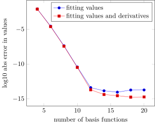

The conclusion is that even without matching them explicitly, derivatives are well-approximated. Getting an extra digit of accuracy in derivatives above 12–14 nodes means sacrificing a digit of accuracy with a low number of nodes. 14 seems to be the break-even point here, but then we are at machine precision anyway.

As usual, simply approximating with Chebyshev polynomials is extremely accurate in itself for practical purposes, even when derivatives are needed. Of course, this depends on the function being “nice”.

By: Tamás K. Papp

Re-posted from: https://tamaspapp.eu/pages/blog/2022/09-14-reproducible-examples/index.html

When migrating this blog recently from Hugo to Franklin.jl, the main difficulty I faced was reproducing old examples (so effectively I didn't rerun anything, and just moved the old generated HTML pages). I have been bothered by this for a long time, so I wrote a quick hack which I packaged up in ReproducibleLiteratePage.jl.

This page was processed using that package. Here is how it works:

1. take a Julia code file marked up with Literate.jl,

2. add a Project.toml and a Manifest.toml (eg activate the directory as a project and add packages)

3. produce a markdown file using ReproducibleLiteratePage.compile_directory().

Here is some code:

using UnPack # the lightest package I could think of
struct Foo
    a
    b
end
@unpack a, b = Foo(1, 2)
a, b

(1, 2)

The Julia source (again, marked up with Literate.jl), Project.toml, and Manifest.toml should be available as a tar archive at the bottom of the page.