By: Dean Markwick's Blog -- Julia
Re-posted from: https://dm13450.github.io/2022/11/18/Trend-Following-with-ETFs.html
Trend following is a rebranded name for momentum trading strategies. It looks at assets where the price has gone up and buying them because it believes the price will continue to rise and likewise for falling prices where it sells. I’ll use this post to show you how to build a basic trend-following strategy in Julia with free market data.
Enjoy these types of posts? Then you should sign up for my newsletter. It’s a short monthly recap of anything and everything I’ve found interesting recently plus
any posts I’ve written. So sign up and stay informed!
Trend following is one of the core quant strategies out there and countless pieces are written, podcasts made, and threads discussed all over Twitter about how to build and use a trend following strategy effectively. This blog post is my exploration of trend-following and uses ETFs to explore the ideas of momentum.
Over the past few months, we have been experiencing the first actual period of sustained volatility and general negative performance across all asset classes. Stocks no longer just go up. This is driven by inflation, the strengthening of the dollar, and the rise in global interest rates it feels like always buying equities 100% isn’t a foolproof plan and diversifying can help. This is where trend following comes in. It wants to try and provide positive returns whether the market is going up or down and, give diversification in regimes like we appear to be in today.
As ever I’ll be using AlpacaMarkets.jl for data and walking you through all the steps. My inspiration comes from the Cantab Capital (now part of GAM) where they had a beautiful blog post doing similar: Trend is not your only friend. Since moving over to the GAM website it no longer looks as good!
using AlpacaMarkets
using DataFrames, DataFramesMeta
using Dates
using Plots, PlotThemes
using RollingFunctions, Statistics
theme(:bright)
ETFs vs Futures in Trend Following
In the professional asset management world trend following is implemented using futures. They are typically cheaper to trade and easier to use leverage. For the average retail investor though, trading futures is a bit more of a headache as you need to roll them as they expire. So ETFs can be the more stress-free option that represents the same underlying.
More importantly, Alpaca Markets has data on ETFs for free whereas I think I would have to pay for the futures market data.
So let’s start by getting the data and preparing it for the strategy.
We will be using three ETFs that represent the different assets classes:
- SPY for stocks
- BND for bonds
- GLD for gold
We expect the three of these ETFs to move in a somewhat independent manner to each other given their different durations, sensitivity to interest rates, and risk profiles.
The stock_bars function from AlpacaMarkets.jl returns the daily OHCL data that we will be working with. You also want to use the adjustment="all" flag so that dividends and stock splits are accounted for.
spy = stock_bars("SPY", "1Day"; startTime = now() - Year(10), limit = 10000, adjustment = "all")[1]
bnd = stock_bars("BND", "1Day"; startTime = now() - Year(10), limit = 10000, adjustment = "all")[1];
gld = stock_bars("GLD", "1Day"; startTime = now() - Year(10), limit = 10000, adjustment = "all")[1];
We do some basic cleaning, formatting the time into a DateTime and just pulling the columns we want, Open, Close Next Open.
function parse_date(t)
   Date(string(split(t, "T")[1]))
end

function clean(df, x)
    df = @transform(df, :Date = parse_date.(:t), :Ticker = x, :NextOpen = [:o[2:end]; NaN])
   @select(df, :Date, :Ticker, :c, :o, :NextOpen)
end

spy = clean(spy, "SPY")
bnd = clean(bnd, "BND")
gld = clean(gld, "GLD");
Joining it all into one long data frame gives us the model data going forward
allPrices = vcat(spy, bnd, gld)
allPrices = sort(allPrices, :Date)
last(allPrices, 6)
6 rows × 5 columns
| Date | Ticker | c | o | NextOpen | |
|---|---|---|---|---|---|
| Date | String | Float64 | Float64 | Float64 | |
| 1 | 2022-10-31 | SPY | 386.21 | 386.44 | 390.14 |
| 2 | 2022-10-31 | BND | 70.35 | 70.36 | 70.58 |
| 3 | 2022-10-31 | GLD | 151.91 | 152.16 | 153.82 |
| 4 | 2022-11-01 | SPY | 384.52 | 390.14 | NaN |
| 5 | 2022-11-01 | BND | 70.26 | 70.58 | NaN |
| 6 | 2022-11-01 | GLD | 153.46 | 153.82 | NaN |
plot(plot(spy.Date, spy.c, label = :none, title = "SPY"),
plot(bnd.Date, bnd.c, label = :none, title = "BND", color = "red"),
plot(gld.Date, gld.c, label = :none, title= "GLD", color = "green"), layout = (3,1))
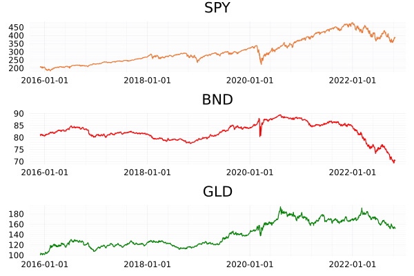
The prices of each ETF are on different scales. BND is between 70-80, GLD in the 100’s and SPY is in the 300-400 range. The scale on which they move is also different. SPY has doubled since 2016, GLD 80% increase, and BND hasn’t done much. Therefore we need to normalise both of these factors to something comparable across all three. To achieve this we first calculate the log-returns of the close-to-close move of each ETF. We then calculate the rolling standard deviation of the price series to represent the volatility which is used to normalise the log returns
\[\hat{r} = 0.1 \frac{\ln p_t – \ln p_{ti}}{\sigma}.\]
allPrices = @transform(groupby(allPrices, :Ticker),
                      :Return = [NaN; diff(log.(:c))],
                      :ReturnTC = [NaN; diff(log.(:NextOpen))]);
We also calculate the returns of using the NextOpen time series as a way to assess the transaction costs of the trend-following strategy, but more on that later.
runvar calculates the 256-day moving variance, which we take the square root of to get the running volatility. There the normalisation step is a simple multiplication and division.
allPrices = @transform(groupby(allPrices, :Ticker), :RunVol = sqrt.(runvar(:Return,  256)));
allPrices = @transform(groupby(allPrices, :Ticker), :rhat = :Return .* 0.1 ./ :RunVol);
Dropping any NaNs removes the data points before we had enough observations for the 256-day volatility calculation and calculating the cumulative sum of the returns gives us an equity curve.
allPricesClean = @subset(allPrices, .!isnan.(:rhat ))
allPricesClean = @transform(groupby(allPricesClean, :Ticker), :rhatC = cumsum(:rhat), :rc = cumsum(:Return));
To check this transformation has worked we aggregate across each ticker.
@combine(groupby(allPricesClean, :Ticker), :AvgReturn = mean(:Return), :AvgNormReturn = mean(:rhat),
                                           :StdReturn = std(:Return), :StdNormReturn = std(:rhat))
3 rows × 5 columns
| Ticker | AvgReturn | AvgNormReturn | StdReturn | StdNormReturn | |
|---|---|---|---|---|---|
| String | Float64 | Float64 | Float64 | Float64 | |
| 1 | SPY | 0.000372633 | 0.00343358 | 0.0122161 | 0.115383 |
| 2 | BND | -9.4164e-5 | -0.00223913 | 0.00349196 | 0.113982 |
| 3 | GLD | 0.000214564 | 0.00288888 | 0.0086931 | 0.101731 |
Summarising the average and standard deviation of the return and normalised return shows the standard deviation is now close to 0.1 as intended.
This is where leverage comes in because bonds have lower volatility than stocks, we have to borrow money to increase the volatility of our bond investment. For example, let’s borrow £100 with £10 of collateral and invest the £100 in BND. If BND moves up by 1% it is now worth £101, we sell and pay back our loan and we are left with £11 which is a 10% return on our original investment. So even though the price only moved by 1% the use of leverage has amplified our return by 10x.
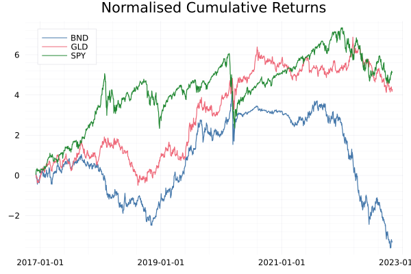
Plotting the cumulative log returns shows how they are on similar scales now.
plot(allPricesClean.Date, allPricesClean.rhatC,
     group = allPricesClean.Ticker, legend=:topleft, title = "Normalised Cumulative Returns")
The Trend Following Signal
With our data in a good shape, we can move on to the actual signal construction. Just like the Cantab article, we will be using the 100-day moving average. Using the RollingFunctions.jl package again we just have to set the window length to 100 and it will do the hard work for us. The actual signal is whether this running average is positive or negative. If it is greater than zero we want to go long as the signal is saying buy. Likewise, if the rolling average is less than zero then we want to go short, the signal is saying sell. So this simply means taking the sign of the rolling average each day.
If we didn’t want to go short, we just want to know when to buy or sell to cover we can simplify it further by just using the signal when it is positive. We will call this the long only signal.
Using data frame manipulation we can calculate the signal per day for each ETF.
allPricesClean = @transform(groupby(allPricesClean, :Ticker),
                            :Signal = sign.(runmean(:rhat, 100)),
                            :SignalLO = runmean(:rhat, 100) .> 0);
Evaluating the Trend Following Strategy
We’ve got our signal that says when to go long and short for each ETF. We need to combine the return of each ETF per day to get out the Trend Following return. As we are using log returns this is as simple as summing across the ETFs multiplied by the signal on each day. We have three ETFs so need to weight each of the returns by 1/3 otherwise when comparing to the single ETFs we would have 3x as much capital invested in the trend following strategy.
portRes = @combine(groupby(allPricesClean, :Date),
           :TotalReturn = sum((1/3)*(:Signal .* :rhat)),
           :TotalReturnLO = sum((1/3)*(:SignalLO .* :rhat)),
           :TotalReturnTC = sum((1/3) * (:Signal .* :ReturnTC)),
           :TotalReturnUL = sum((1/3) * (:Signal .* :Return)));
Again, plotting the cumulative returns shows that this trend-following strategy (dark blue) is great. I’ve massively outperformed just being long the SPY ETF. Even when we remove the shorting element (Trend Following – LO, red) this has done well.
portRes = @transform(portRes, :TotalReturnC = cumsum(:TotalReturn),
                              :TotalReturnLOC = cumsum(:TotalReturnLO),
                              :TotalReturnTCC = cumsum(:TotalReturnTC),
                              :TotalReturnULC = cumsum(:TotalReturnUL))

plot(portRes.Date, portRes.TotalReturnC, label = "Trend Following", legendposition = :topleft, linewidth=3)
plot!(portRes.Date, portRes.TotalReturnLOC, label = "Trend Following - LO", legendposition = :topleft, linewidth=3)

plot!(allPricesClean.Date, allPricesClean.rhatC, group = allPricesClean.Ticker)
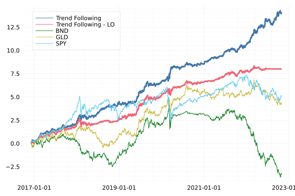
It’s up and to the right which is a good sign. By following the trends in the market we can profit when it is both going up and down. This is without any major sophistication on predicting the direction either. Simply using the average produces enough of a signal to be profitable.
Let’s focus on just what has happened this year
portRes2022 = @transform(@subset(portRes, :Date .>= Date("2022-01-01")),
            :TotalReturnC = cumsum(:TotalReturn),
            :TotalReturnLOC = cumsum(:TotalReturnLO),
            :TotalReturnULC = cumsum(:TotalReturnUL))

allPricesClean2022 = @subset(allPricesClean, :Date .>= Date("2022-01-01"))
allPricesClean2022 = @transform(groupby(allPricesClean2022, :Ticker), :rhatC = cumsum(:Return))

plot(portRes2022.Date, portRes2022.TotalReturnULC, label = "Trend Following", legendposition = :topleft, linewidth = 3)
plot!(portRes2022.Date, portRes2022.TotalReturnLOC, label = "Trend Following - LO", legendposition = :topleft, linewidth =3)
plot!(allPricesClean2022.Date, allPricesClean2022.rhatC, group = allPricesClean2022.Ticker)
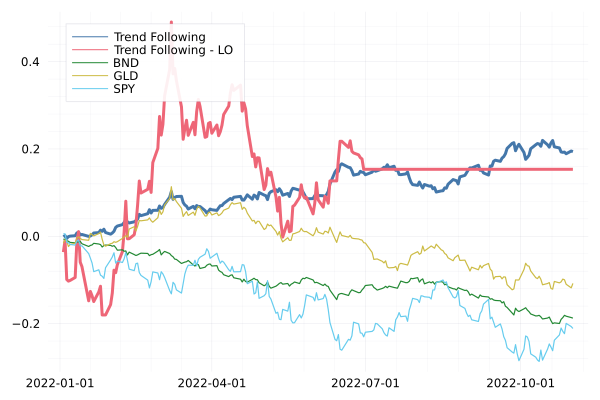
The long-only (red line) staying flat is indicating that we’ve been out of the market since July. The trend-following strategy has been helped by the fact that it is all one-way traffic in the markets at the minute. It’s just been heading lower and lower across all the asset classes since the summer.
Implementation Shortfall and Thinking Practically
Everything above looks like a decent trend-following approach. But how do we implement this, or simulate an implementation? By this, I mean obtaining the trades that should be made.
The mechanics of this strategy are simple:
- Calculate the close-to-close return of an ETF
- If it is above the 100-day moving average buy, if it’s below sell or go short.
The price we can trade at though is not the close price, markets are closed, and you can’t place any more orders! Instead, you will be buying at the open on the next day. So whilst our signal has triggered, our actual price is different from the theoretical price.
Sidenote, it is possible to trade after hours, and in the small size, you might be able to get close to the closing price.
Given this is retail and the sizes are so small, we are going to assume I get the next day’s open price. We can compare our purchase price to the model price. The difference between the two is called ‘Implementation Shortfall’ and measures how close you traded relative to the actual price you wanted to trade.
If we are buying higher than the model price (or selling lower) we are missing out on some of the moves and it’s going to eat the performance of the strategy.
To calculate this Implementation Shortfall (IS) we pull out the days where the signal changed, as this indicates a trade needs to be made.
allPricesClean = @transform(groupby(allPricesClean, :Ticker), :SigChange = [NaN; diff(:Signal)])

trades = @subset(allPricesClean[!, [:Date, :Ticker, :o, :c, :Signal, :NextOpen, :SigChange]],
             :SigChange .!= 0);
Then by calculating the difference between the next open and closing price we have our estimation of the IS value.
@combine(groupby(trades, :Ticker),
        :N = length(:Signal),
        :IS = mean(:Signal .* 1e4 .* (:NextOpen .- :c) ./ :c))
3 rows × 3 columns
| Ticker | N | IS | |
|---|---|---|---|
| String | Int64 | Float64 | |
| 1 | SPY | 40 | 14.7934 |
| 2 | BND | 69 | -6.45196 |
| 3 | GLD | 61 | 10.4055 |
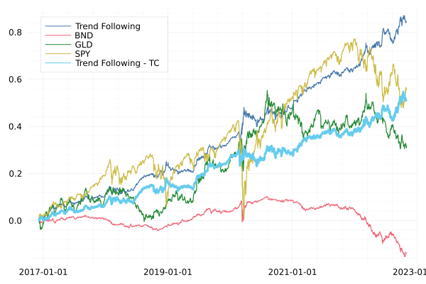
For both SPY and GLD we have lost 15bps and 10bps to this difference between the close and the next open. For BND though we actually would earn more than the close price, again, this is down to the one-way direction of bonds this year. But overall, implementation shortfall is a big drag on returns. We can plot the equity curve including this transaction cost.
plot(portRes.Date, portRes.TotalReturnULC, label = "Trend Following", legendposition = :topleft)
plot!(allPricesClean.Date, allPricesClean.rc, group = allPricesClean.Ticker)
plot!(portRes.Date, portRes.TotalReturnTCC, label = "Trend Following - TC", legendposition = :topleft, linewidth = 3)
What’s the old saying:
“In theory there is no difference between theory and practice – in practice there is” (Yogi Berra)
Implementation shortfall is just one transaction cost. There are also actual physical costs to consider too:
- Brokerage costs
- Borrow fees
- Capacity
Let’s start with the simple transaction costs. Each time you buy or sell you are probably paying some sort of small fee. At Interactive Brokers, it is $0.005 with a minimum of $1. So if you trade $100 of one of the ETFs you will be paying 1\% in feeds. You could get rid of this fee completely with a free broker like Robinhood which is one way to keep the costs down.
This model requires you to go short the different ETFs, so you will also need to pay borrow fees to whoever you borrow the ETF from. This is free for up to $100k in Interactive Brokers, so not a concern for the low-capacity retail trader. You can’t short sell on Robinhood directly, instead, you’ll have to use options or inverse ETFs which is just complicating matters and overall not going to bring costs down.
All these fees mean there is both a minimum amount and a maximum amount that you can implement this model with. If you have too small of a budget your returns will just be eaten up by transaction costs. If you have a large amount of money, the implementation shortfall hurts. This is what we mean by capacity.
Next Steps in Trend Following
The above implementation is the most basic possible trend following. It only uses three assets when there is a whole world of other ETFs out there. It has a simple signal (running average) and uses that to either allocate 100% long or 100% short. There are several ways in which you can go further to make this better.
- Expand the asset universe.
Including more ETFs and ones that are uncorrelated to SPY, BND and GLD gives you a broader opportunity to go long or short. I would look at including some sort of commodity, real estate, and international equity component as the next ETFs.
- A better trend signal.
The simple moving average is great as there are no moving parts, but nothing is stopping it from being expanded to a more sophisticated model. Including another moving average with a faster period, say 5 days, and then checking as to whether this faster average is higher or lower than the slow average is also commonly used.
- Better asset allocation using the signal
The current signal says {-1, 1} and no in-between. This can lead to some volatile behaviour where the signal might be hovering around 0 and leading to going long and short quickly around multiple days. Instead, you should map the signal strength onto a target position with some sort of function. This could mean waiting for the signal to get strong enough before trading and then linearly adding to the position until you max out the allocation.
Conclusion
Trend following is a profitable strategy. We’ve shown that using a simple rolling average of the returns can produce a profitable signal. When scrutinising it a bit further we find that it is difficult to achieve these types of returns in practise. The overnight price movements in the ETFs means that we trade at a worse price. This combined with the general transaction costs of making the trades makes it a hard strategy to implement and to rely on another quote, there is no such thing as a free lunch, you have to put in a remarkable amount of effort to scale this kind of strategy up. We then highlight several ways you could take this research further. So you now have everything at your fingertips to explore Trend Following yourself. Let me know anything I’ve missed in the comments below.
