Category Archives: Julia

Julia’s Parallel Processing

By: Steven Whitaker

Re-posted from: https://glcs.hashnode.dev/parallel-processing

Julia is a relatively new, free, and open-source programming language. It has a syntax similar to that of other popular programming languages such as MATLAB and Python, but it boasts being able to achieve C-like speeds.

While serial Julia code can be fast, sometimes even more speed is desired. In many cases, writing parallel code can further reduce run time. Parallel code takes advantage of the multiple CPU cores included in modern computers, allowing multiple computations to run at the same time, or in parallel.

Julia provides two methods for writing parallel CPU code: multi-threading and distributed computing. This post will cover the basics of how to use these two methods of parallel processing.

This post assumes you already have Julia installed. If you haven’t yet, check out our earlier post on how to install Julia.

Multi-Threading

First, let’s learn about multi-threading.

To enable multi-threading, you must start Julia in one of two ways:

  1. Set the environment variable JULIA_NUM_THREADS to the number of threads Julia should use, and then start Julia. For example, JULIA_NUM_THREADS=4.

  2. Run Julia with the --threads (or -t) command line argument. For example, julia --threads 4 or julia -t 4.

After starting Julia (either with or without specifying the number of threads), the Threads module will be loaded. We can check the number of threads Julia has available:
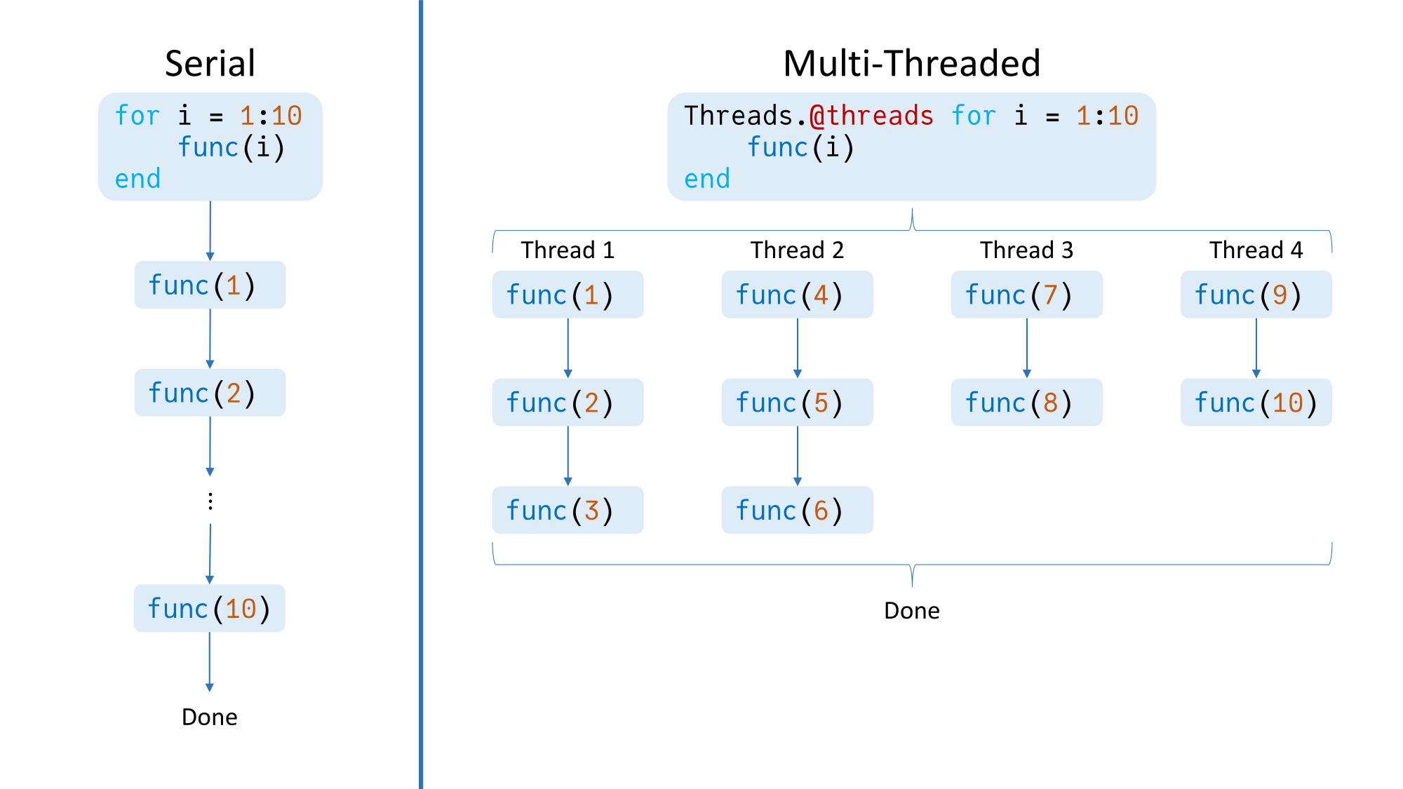
julia> Threads.nthreads()4

The simplest way to start writing parallel code is just to use the Threads.@threads macro. Inserting this macro before a for loop will cause the iterations of the loop to be split across the available threads, which will then operate in parallel. For example:

Threads.@threads for i = 1:10    func(i)end

Without Threads.@threads, first func(1) will run, then func(2), and so on. With the macro, and assuming we started Julia with four threads, first func(1), func(4), func(7), and func(9) will run in parallel. Then, when a thread’s iteration finishes, it will start another iteration (assuming the loop is not done yet), regardless of whether the other threads have finished their iterations yet. Therefore, this loop will theoretically finish 10 iterations in the time it takes a single thread to do 3.

Note that Threads.@threads is blocking, meaning code after the threaded for loop will not run until the loop has finished.

Image of threaded for loop

threads_for

Julia also provides another macro for multi-threading: Threads.@spawn. This macro is more flexible than Threads.@threads because it can be used to run any code on a thread, not just for loops. But let’s illustrate how to use Threads.@spawn by implementing the behavior of Threads.@threads:

# Function for splitting up `x` as evenly as possible# across `np` partitions.function partition(x, np)    (len, rem) = divrem(length(x), np)    Base.Generator(1:np) do p        i1 = firstindex(x) + (p - 1) * len        i2 = i1 + len - 1        if p <= rem            i1 += p - 1            i2 += p        else            i1 += rem            i2 += rem        end        chunk = x[i1:i2]    endendN = 10chunks = partition(1:10, Threads.nthreads())tasks = map(chunks) do chunk    Threads.@spawn for i in chunk        func(i)    endendwait.(tasks)

Let’s walk through this code, assuming Threads.nthreads() == 4:

  • First, we split the 10 iterations evenly across the 4 threads using partition. So, chunks ends up being [1:3, 4:6, 7:8, 9:10]. (We could have hard-coded the partitioning, but now you have a nice partition function that can work with more complicated partitionings!)

  • Then, for each chunk, we create a Task via Threads.@spawn that will call func on each element of the chunk. This Task will be scheduled to run on an available thread. tasks contains a reference to each of these spawned Tasks.

  • Finally, we wait for the Tasks to finish with the wait function.

To reemphasize, note that Threads.@spawn creates a Task; it does not wait for the task to run. As such, it is non-blocking, and program execution continues as soon as the Task is returned. The code wrapped in the task will also run, but in parallel, on a separate thread. This behavior is illustrated below:

julia> Threads.@spawn (sleep(2); println("Spawned task finished"))Task (runnable) @0x00007fdd4b10dc30julia> 1 + 1 # This code executes without waiting for the above task to finish2julia> Spawned task finished # Prints 2 seconds after spawning the above taskjulia>

Spawned tasks can also return data. While wait just waits for a task to finish, fetch waits for a task and then obtains the result:

julia> task = Threads.@spawn (sleep(2); 1 + 1)Task (runnable) @0x00007fdd4a5e28b0julia> fetch(task)2

Thread Safety

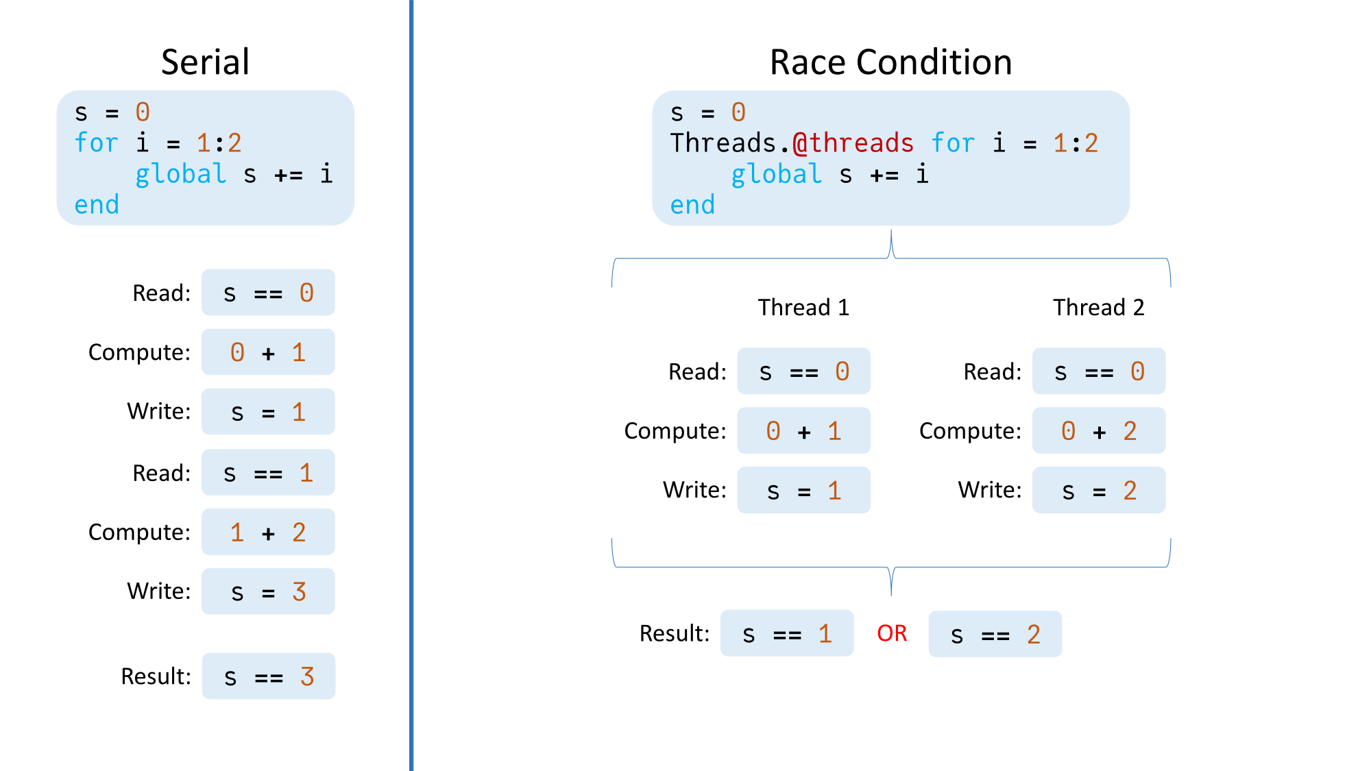
When using multi-threading, memory is shared across threads. If a thread writes to a memory location that is written to or read from another thread, that will lead to a race condition with unpredictable results. To illustrate:

julia> s = 0;julia> Threads.@threads for i = 1:1000000           global s += i       endjulia> s19566554653 # Should be 500000500000

Race condition

race_condition

There are two methods we can use to avoid the race condition. The first involves using a lock:

julia> s = 0; l = ReentrantLock();julia> Threads.@threads for i = 1:1000000           lock(l) do               global s += i           end       endjulia> s500000500000

In this case, the addition can only occur on a given thread once that thread holds the lock. If a thread does not hold the lock, it must wait for whatever thread controls it to release the lock before it can run the code within the lock block.

Using a lock in this example is suboptimal, however, as it eliminates all parallelism because only one thread can hold the lock at any given moment. (In other examples, however, using a lock works great, particularly when only a small portion of the code depends on the lock.)

The other way to eliminate the race condition is to use task-local buffers:

julia> s = 0; chunks = partition(1:1000000, Threads.nthreads());julia> tasks = map(chunks) do chunk           Threads.@spawn begin               x = 0               for i in chunk                   x += i               end               x           end       end;julia> thread_sums = fetch.(tasks);julia> for i in thread_sums           s += i       endjulia> s500000500000

In this example, each spawned task has its own x that stores the sum of the values just in the task’s chunk of data. In particular, none of the tasks modify s. Then, once each task has computed its sum, the intermediate values are summed and stored in s in a single-threaded manner.

Using task-local buffers works better for this example than using a lock because most of the parallelism is preserved.

(Note that it used to be advised to manage task-local buffers using the threadid function. However, doing so does not guarantee each task uses its own buffer. Therefore, the method demonstrated in the above example is now advised.)

Packages for Quickly Utilizing Multi-Threading

In addition to writing your own multi-threaded code, there exist packages that utilize multi-threading. Two such examples are ThreadsX.jl and ThreadTools.jl.

ThreadsX.jl provides multi-threaded implementations of several common functions such as sum and sort, while ThreadTools.jl provides tmap, a multi-threaded version of map.

These packages can be great for quickly boosting performance without having to figure out multi-threading on your own.

Distributed Computing

Besides multi-threading, Julia also provides for distributed computing, or splitting work across multiple Julia processes.

There are two ways to start multiple Julia processes:

  1. Load the Distributed standard library package with using Distributed and then use addprocs. For example, addprocs(2) to add two additional Julia processes (for a total of three).

  2. Run Julia with the -p command line argument. For example, julia -p 2 to start Julia with three total Julia processes. (Note that running Julia with -p will implicitly load Distributed.)

Added processes are known as worker processes, while the original process is the main process. Each process has an id: the main process has id 1, and worker processes have id 2, 3, etc.

By default, code runs on the main process. To run code on a worker, we need to explicitly give code to that worker. We can do so with remotecall_fetch, which takes as inputs a function to run, the process id to run the function on, and the input arguments and keyword arguments the function needs. Here are some examples:

# Create a zero-argument anonymous function to run on worker 2.julia> remotecall_fetch(2) do           println("Done")       end      From worker 2:    Done# Create a two-argument anonymous function to run on worker 2.julia> remotecall_fetch((a, b) -> a + b, 2, 1, 2)3# Run `sum([1 3; 2 4]; dims = 1)` on worker 3.julia> remotecall_fetch(sum, 3, [1 3; 2 4]; dims = 1)1x2 Matrix{Int64}: 3  7

If you don’t need to wait for the result immediately, use remotecall instead of remotecall_fetch. This will create a Future that you can later wait on or fetch (similarly to a Task spawned with Threads.@spawn).

Super computer

super_computer

Separate Memory Spaces

One significant difference between multi-threading and distributed processing is that memory is shared in multi-threading, while each distributed process has its own separate memory space. This has several important implications:

  • To use a package on a given worker, it must be loaded on that worker, not just on the main process. To illustrate:

      julia> using LinearAlgebra  julia> I  UniformScaling{Bool}  true*I  julia> remotecall_fetch(() -> I, 2)  ERROR: On worker 2:  UndefVarError: `I` not defined

    To avoid the error, we could use @everywhere using LinearAlgebra to load LinearAlgebra on all processes.

  • Similarly to the previous point, functions defined on one process are not available on other processes. Prepend a function definition with @everywhere to allow using the function on all processes:

      julia> @everywhere function myadd(a, b)             a + b         end;  julia> myadd(1, 2)  3  # This would error without `@everywhere` above.  julia> remotecall_fetch(myadd, 2, 3, 4)  7
  • Global variables are not shared, even if defined everywhere with @everywhere:

      julia> @everywhere x = [0];  julia> remotecall_fetch(2) do             x[1] = 2         end;  # `x` was modified on worker 2.  julia> remotecall_fetch(() -> x, 2)  1-element Vector{Int64}:   2  # `x` was not modified on worker 3.  julia> remotecall_fetch(() -> x, 3)  1-element Vector{Int64}:   0

    If needed, an array of data can be shared across processes by using a SharedArray, provided by the SharedArrays standard library package:

      julia> @everywhere using SharedArrays  # We don't need `@everywhere` when defining a `SharedArray`.  julia> x = SharedArray{Int,1}(1)  1-element SharedVector{Int64}:   0  julia> remotecall_fetch(2) do             x[1] = 2         end;  julia> remotecall_fetch(() -> x, 2)  1-element SharedVector{Int64}:   2  julia> remotecall_fetch(() -> x, 3)  1-element SharedVector{Int64}:   2

Now, a note about command line arguments. When adding worker processes with -p, those processes are spawned with the same command line arguments as the main Julia process. With addprocs, however, each of those added processes are started with no command line arguments. Below is an example of where this behavior might cause some confusion:

$ JULIA_NUM_THREADS=4 julia --banner=no -t 1julia> Threads.nthreads()1julia> using Distributedjulia> addprocs(1);julia> remotecall_fetch(Threads.nthreads, 2)4

In this situation, we have the environment variable JULIA_NUM_THREADS (for example, because normally we run Julia with four threads). But in this particular case we want to run Julia with just one thread, so we set -t 1. Then we add a process, but it turns out that process has four threads, not one! This is because the environment variable was set, but no command line arguments were given to the added process. To use just one thread for the added process, we would need to use the exeflags keyword argument to addprocs:

addprocs(1; exeflags = ["-t 1"])

As a final note, if needed, processes can be removed with rmprocs, which removes the processes associated with the provided worker ids.

Summary

In this post, we have provided an introduction to parallel processing in Julia. We discussed the basics of both multi-threading and distributed computing, how to use them in Julia, and some things to watch out for.

As a parting piece of advice, when choosing whether to use multi-threading or distributed processing, choose multi-threading unless you have a specific need for multiple processes with distinct memory spaces. Multi-threading has lower overhead and generally is easier to use.

How do you use parallel processing in your code? Let us know in the comments below!

Additional Links

What to do when you are stuck with Julia?

By: Blog by Bogumił Kamiński

Re-posted from: https://bkamins.github.io/julialang/2024/01/12/rgg.html

Introduction

Today I decided to write about code refactoring in Julia.
This is a topic that is, in my experience, a quite big advantage of this language.

A common situation you are faced with when writing your code is as follows.
You need some functionality in your program and it is available in some library.
However, what the library provides does not meet your expectations.
Since in Julia most packages are written in Julia under MIT license, it is easy to solve this issue.
You just take the source code and modify it.

Today I want to show you a practical example of such a situation I have had this week
when working with the Graphs.jl package.

The post was written using Julia 1.10.0, BenchmarkTools.jl 1.4.0, and Graphs.jl 1.9.0.

The problem

In my work I needed to generate random geometric graphs.
This is a simple random graph model that works as follows
(here I describe a general idea, for details please check the
Wikipedia entry on random geometric graphs).
To generate a graph on N vertices you first drop N random points
in some metric space. Next you connect two points with an edge
if their distance is less than some pre-specified distance.

The Graphs.jl library provides the euclidean_graph function
that generates such graphs. Here is a summary of its docstring:

euclidean_graph(N, d; rng=nothing, seed=nothing, L=1., p=2., cutoff=-1., bc=:open)

Generate N uniformly distributed points in the box [0,L]^{d}
and return a Euclidean graph, a map containing the distance on each
edge and a matrix with the points' positions.

An edge between vertices x[i] and x[j] is inserted if norm(x[i]-x[j], p) < cutoff.
In case of negative cutoff instead every edge is inserted.
Set bc=:periodic to impose periodic boundary conditions in the box [0,L]^d.

So what is the problem with this function? Unfortunately it is slow.
Let us, for example check how long it takes to compute an average degree
of a node in such a graph with n nodes and cutoff=sqrt(10/n), when setting
bc=:periodic (periodic boundary, i.e. distance is measured on a torus) for two-dimensional space.

julia> using Graphs

julia> for n in 1_000:1_000:10_000
           println(@time ne(euclidean_graph(n, 2; cutoff=sqrt(10/n), bc=:periodic, seed=1)[1])/n)
       end
  0.091657 seconds (2.50 M allocations: 193.170 MiB, 14.06% gc time)
15.604
  0.300285 seconds (10.00 M allocations: 765.801 MiB, 12.59% gc time)
15.661
  0.686230 seconds (22.50 M allocations: 1.686 GiB, 12.47% gc time)
15.744
  1.175881 seconds (40.00 M allocations: 2.990 GiB, 10.97% gc time)
15.7065
  1.800561 seconds (62.50 M allocations: 4.666 GiB, 10.76% gc time)
15.6568
  2.697535 seconds (90.00 M allocations: 6.716 GiB, 14.76% gc time)
15.641333333333334
  3.690599 seconds (122.50 M allocations: 9.138 GiB, 13.28% gc time)
15.743571428571428
  4.745701 seconds (160.00 M allocations: 11.932 GiB, 13.53% gc time)
15.714
  5.962431 seconds (202.51 M allocations: 15.099 GiB, 12.70% gc time)
15.722222222222221
  7.195257 seconds (250.01 M allocations: 18.638 GiB, 11.42% gc time)
15.7086

We can see that the euclidean_graph function scales badly with n.
Note that by choosing cutoff=sqrt(10/n) we have a roughly constant
average degree, so the number of edges generates scales linearly, but
the generation time seems to grow much faster.

The investigation

To find out the source of the problem we can investigate the source
of euclidean_graph, which consists of two methods:

function euclidean_graph(
    N::Int,
    d::Int;
    L=1.0,
    rng::Union{Nothing,AbstractRNG}=nothing,
    seed::Union{Nothing,Integer}=nothing,
    kws...,
)
    rng = rng_from_rng_or_seed(rng, seed)
    points = rmul!(rand(rng, d, N), L)
    return (euclidean_graph(points; L=L, kws...)..., points)
end

function euclidean_graph(points::Matrix; L=1.0, p=2.0, cutoff=-1.0, bc=:open)
    d, N = size(points)
    weights = Dict{SimpleEdge{Int},Float64}()
    cutoff < 0.0 && (cutoff = typemax(Float64))
    if bc == :periodic
        maximum(points) > L && throw(
            DomainError(maximum(points), "Some points are outside the box of size $L")
        )
    end
    for i in 1:N
        for j in (i + 1):N
            if bc == :open
                Δ = points[:, i] - points[:, j]
            elseif bc == :periodic
                Δ = abs.(points[:, i] - points[:, j])
                Δ = min.(L .- Δ, Δ)
            else
                throw(ArgumentError("$bc is not a valid boundary condition"))
            end
            dist = norm(Δ, p)
            if dist < cutoff
                e = SimpleEdge(i, j)
                weights[e] = dist
            end
        end
    end
    g = Graphs.SimpleGraphs._SimpleGraphFromIterator(keys(weights), Int)
    if nv(g) < N
        add_vertices!(g, N - nv(g))
    end
    return g, weights
end

The beauty of Julia is that this source is written in Julia and is pretty short.
It immediately allows us to pinpoint the source of our problems. The core of we work
is done in a double-loop iterating over i and j indices. So the complexity of this
algorithm is quadratic in number of vertices.

Fixing the problem

The second beauty of Julia is that we can easily fix this. The idea can be found in
the Wikipedia entry on random geometric graphs in the algorithms section
here.

A simple way to improve the performance of the algorithm is to notice that if
you know L and cutoff you can partition the space into equal sized cells
having side length floor(Int, L / cutoff). Now you see that if you have a vertex
in some cell then it can be connected only to nodes in the same cell or cells directly
adjacent to it (the cells that are more far away contain the points that must be farther
than cutoff from our point). This means that we will have a much lower number of points
to consider. Below I show a code that is a modification of the original source that
adds this feature. The key added function is to_buckets which computes the bucket
identifier for each vertex and creates a dictionary that is a mapping from bucked
identifier to a vector of node numbers that fall into it:

using LinearAlgebra
using Random

function euclidean_graph2(
    N::Int,
    d::Int;
    L=1.0,
    rng::Union{Nothing,AbstractRNG}=nothing,
    seed::Union{Nothing,Integer}=nothing,
    kws...,
)
    rng = Graphs.rng_from_rng_or_seed(rng, seed)
    points = rmul!(rand(rng, d, N), L)
    return (euclidean_graph2(points; L=L, kws...)..., points)
end

function to_buckets(points::Matrix, L, cutoff)
    d, N = size(points)
    dimlen = max(floor(Int, L / max(cutoff, eps())), 1)
    buckets = Dict{Vector{Int}, Vector{Int}}()
    for (i, point) in enumerate(eachcol(points))
        bucket = floor.(Int, point .* dimlen ./ L)
        push!(get!(() -> Int[], buckets, bucket), i)
    end
    return buckets, dimlen
end

function euclidean_graph2(points::Matrix; L=1.0, p=2.0, cutoff=-1.0, bc=:open)
    d, N = size(points)
    weights = Dict{Graphs.SimpleEdge{Int},Float64}()
    cutoff < 0.0 && (cutoff = typemax(Float64))
    if bc == :periodic
        maximum(points) > L && throw(
            DomainError(maximum(points), "Some points are outside the box of size $L")
        )
    end
    buckets, dimlen = to_buckets(points, L, cutoff)
    deltas = collect(Iterators.product((-1:1 for _ in 1:size(points, 1))...))
    void = Int[]
    for (k1, v1) in pairs(buckets)
        for i in v1
            for d in deltas
                k2 = bc == :periodic ? mod.(k1 .+ d, dimlen) : k2 = k1 .+ d
                v2 = get(buckets, k2, void)
                for j in v2
                    i < j || continue
                    if bc == :open
                        Δ = points[:, i] - points[:, j]
                    elseif bc == :periodic
                        Δ = abs.(points[:, i] - points[:, j])
                        Δ = min.(L .- Δ, Δ)
                    else
                        throw(ArgumentError("$bc is not a valid boundary condition"))
                    end
                    dist = norm(Δ, p)
                    if dist < cutoff
                        e = Graphs.SimpleEdge(i, j)
                        weights[e] = dist
                    end
                end
            end
        end
    end

    g = Graphs.SimpleGraphs._SimpleGraphFromIterator(keys(weights), Int)
    if nv(g) < N
        add_vertices!(g, N - nv(g))
    end
    return g, weights
end

Note that it took less than 30 lines of code to add the requested feature to the code.

Performance of the improved code

Let us test our new code:

julia> for n in 1_000:1_000:10_000
           println(@time ne(euclidean_graph2(n, 2; cutoff=sqrt(10/n), bc=:periodic, seed=1)[1])/n)
       end
  0.017221 seconds (274.10 k allocations: 21.751 MiB, 22.15% gc time)
15.604
  0.022855 seconds (558.52 k allocations: 42.289 MiB, 10.43% gc time)
15.661
  0.032693 seconds (852.46 k allocations: 69.684 MiB, 8.52% gc time)
15.744
  0.043141 seconds (1.10 M allocations: 87.196 MiB, 14.73% gc time)
15.7065
  0.071273 seconds (1.41 M allocations: 109.725 MiB, 7.67% gc time)
15.6568
  0.068194 seconds (1.70 M allocations: 130.828 MiB, 12.54% gc time)
15.641333333333334
  0.071277 seconds (1.98 M allocations: 150.712 MiB, 11.85% gc time)
15.743571428571428
  0.081463 seconds (2.24 M allocations: 169.153 MiB, 10.67% gc time)
15.714
  0.099957 seconds (2.48 M allocations: 186.492 MiB, 8.08% gc time)
15.722222222222221
  0.148573 seconds (2.84 M allocations: 213.214 MiB, 18.37% gc time)
15.7086

We seem to get what we wanted. Our computation time looks to scale quite well.
Also the obtained average degree numbers are identical to the original ones.

Let us compare the performance on an even larger graph:

julia> n = 100_000;

julia> @time ne(euclidean_graph(n, 2; cutoff=sqrt(10/n), bc=:periodic, seed=1)[1])/n
908.976252 seconds (25.00 G allocations: 1.819 TiB, 11.64% gc time, 0.00% compilation time)
15.70797

julia> julia> @time ne(euclidean_graph2(n, 2; cutoff=sqrt(10/n), bc=:periodic, seed=1)[1])/n
  1.640495 seconds (27.53 M allocations: 2.121 GiB, 19.83% gc time)
15.70797

Indeed we see that the timing of the original implementation becomes prohibitive for
larger graphs.

Making sure things are correct

Before we finish there is one important task we need to make. We should check if
indeed the euclidean_graph2 function produces the same results as euclidean_graph.
This is easy to test with the following randomized test:

julia> using Test

julia> Random.seed!(1234);

julia> @time for i in 1:1000
           N = rand(10:500)
           d = rand(1:5)
           L = rand()
           p = 3*rand()
           cutoff = rand() * L / 4
           bc = rand([:open, :periodic])
           seed = rand(UInt32)
           @test euclidean_graph(N, d; L, p, cutoff, bc, seed) ==
                 euclidean_graph2(N, d; L, p, cutoff, bc, seed)
       end
 16.955773 seconds (275.09 M allocations: 20.342 GiB, 12.27% gc time)

We have tested 1000 random setups of the experiments. In each of them both functions
returned the same results.

Conclusions

In my post I have shown you an example that one can easily tweak some package code to your needs.
In this case this was performance, but it can be equally well functionality.

I did not comment too much on the code itself, as it was a bit longer than usual, but let me
discuss as a closing remark one performance aspect of the code. In my to_buckets function I used
the get! function to populate the dictionary with a mutable default value (Int[] in that case).
You might wonder why I preferred to use an anonymous function instead of passing a default
as a third argument. The reason is number of allocations. Check this code:

julia> using BenchmarkTools

julia> function f1()
           d = Dict(1 => Int[])
           for i in 1:10^6
               get!(d, 1, Int[])
           end
           return d
       end
f1 (generic function with 1 method)

julia> function f2()
           d = Dict(1 => Int[])
           for i in 1:10^6
               get!(() -> Int[], d, 1)
           end
           return d
       end
f2 (generic function with 1 method)

julia> @benchmark f1()
BenchmarkTools.Trial: 195 samples with 1 evaluation.
 Range (min … max):  19.961 ms … 45.328 ms  ┊ GC (min … max): 10.26% … 13.19%
 Time  (median):     23.962 ms              ┊ GC (median):    10.45%
 Time  (mean ± σ):   25.660 ms ±  5.050 ms  ┊ GC (mean ± σ):  12.27% ±  3.76%

    ▃▂▂█▃▃ ▃▂▃
  ▆▄██████▇███▇▆▄▄▇▄▄▁▃▆▄▃▅▄▅▄▄▄▃▄▃▁▃▃▁▁▁▃▃▃▃▃▃▁▃▁▁▃▁▁▁▁▁▃▁▁▃ ▃
  20 ms           Histogram: frequency by time        44.3 ms <

 Memory estimate: 61.04 MiB, allocs estimate: 1000005.

julia> @benchmark f2()
BenchmarkTools.Trial: 902 samples with 1 evaluation.
 Range (min … max):  4.564 ms … 11.178 ms  ┊ GC (min … max): 0.00% … 0.00%
 Time  (median):     5.149 ms              ┊ GC (median):    0.00%
 Time  (mean ± σ):   5.526 ms ±  1.396 ms  ┊ GC (mean ± σ):  0.00% ± 0.00%

  █▅▄▄▃▃▄▅▆▄▁▁                                           ▃
  ██████████████▆▆▆▆▆▅▇▆▄▆▆▅▅▁▄▅▁▅▁▇▅▆▄▄▇▁▅▅▅▄▁▄▄▆▅▁▅▁▁▅▆██▅ █
  4.56 ms      Histogram: log(frequency) by time       10 ms <

 Memory estimate: 592 bytes, allocs estimate: 5.

As you can see f2 is much faster than f1 and does much less allocations. The issue
is that f1 allocates a fresh Int[] object in every iteration of the loop, while
f2 would allocate it only if get! does not hit a key that already exists in d
(and in our experiment I always queried for 1 which was present in d).

Build a Data-Rich Dashboard App on JuliaHub

By: Michael Bologna

Re-posted from: https://info.juliahub.com/blog/build-a-data-rich-dashboard-app-on-juliahub

Software Developers, scientists, R&D teams, and professionals across disciplines, all need a quick and easy way to build visualizations and dashboards that present their research findings to business stakeholders. JuliaHub now offers a swift and effective solution through a hosted web server, providing a platform to host web applications tailored for this purpose.