Category Archives: Julia

Digital Echo: A Process-Centric Approach to Industrial Surrogate Modeling

Re-posted from: https://info.juliahub.com/blog/digital-echo-industrial-surrogate-modeling

Navigating the Surrogates Problem in Industrial Modeling: Towards Process-Driven Precision

Industrial surrogate modeling is typically centered around neural network architectures and precision. While important, these approaches don’t necessarily solve the ‘surrogates problem’. The ‘surrogates problem’ refers to the challenges associated with integrating surrogate models into industrial processes and requirements infrastructure. The challenge with this approach is that it doesn’t integrate surrogates into industrial processes and requirements infrastructure. For surrogate modeling to truly solve real-world industrial engineering problems, verification and validation benchmarks are equally important. This blog post looks at the three key pillars to create surrogates that are process-driven, reliable, and prioritize prediction time for varied industrial applications.

My First Julia Package – TriangulArt.jl

By: Jonathan Carroll

Re-posted from: https://jcarroll.com.au/2024/02/04/my-first-julia-package-triangulart-jl/

I’ve tried to get this same image transformation working at least three times now, but
I can finally celebrate that it’s working! I’ve been (re-)learning Julia and I still
love the language, so it was time to take my learning to the next level and actually
build a package.

For those not familiar, Julia is a much newer language than my daily-driver R, and with
that comes the freedom to take a lot of good features from other languages and implement
them. There are some features that R just won’t ever get, but they’re available in Julia and
they’re very nice to use.

I’ve written solutions to the first 20
or so Project Euler problems in Julia … wow, 5 years ago.

More recently, I have solved the first 18 days of Advent of Code 2023 in Julia
(my solutions
are in a fork of a package that I’m not using, so they more or less run independently).

With those under my belt, I revisited a project I’ve tried to implement several times. I like
the low-poly look and wanted to recreate it – it’s just an image transformation,
right? I’m even somewhat familiar with Delaunay Triangulation, or at least its dual the
Voronoi Tesselation from my days building spatial maps
of fishing areas.

It sounds like a simple enough problem; choose some points all over the image, triangulate between
all of them, then shade the resulting triangles with the average colour of the pixels they enclose.

I found this nice image of a rainbow lorikeet (these frequent my backyard)

Rainbow Lorikeet

so I got to work trying to chop it up into triangles.

Well, the naive approach is simple enough, but it produces some terrible results. I’ve built that version into what I did eventually get working, and it’s… not what I want

It works, but at what cost?

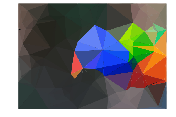
The problem is that by randomly selecting points across the image, you lose all the structure. With
enough triangles you might recover some of that, but then you have a lot of triangles and lose that
low-poly vibe.

After much searching for a better way to do this, I found this article from 2017. It’s
a python approach, but I figured I knew enough Julia and Python now that I could try to make
a 1:1 translation.

The first step is to get the random sampling working, because it allows me to start testing
the triangulation parts quickly. Generating those is pretty clean

function generate_uniform_random_points(image::Matrix{RGB{N0f8}}, n_points::Integer=100)
    ymax, xmax = size(image)[1:2]
    rand(n_points, 2) .* [xmax ymax]
end

The triangulation itself is handled by DelaunayTriangulation::triangulate() –
for once I’m happy that there’s so much scientific/statistical support in Julia

rng = StableRNG(2)
tri = triangulate(all_points; rng)

Slightly trickier is figuring out which points are in which triangle. For that, I am
thankful for PolygonOps::inpolygon(). With the pixels for each triangle identified,
it was only a matter of averaging the R, G, and B channels to get the median colour.

I got that working, but with the results above – far from pleasant. The next, much harder step,
was to weight the points towards the ’edges’ of the image. I couldn’t find an easy
way to translate the python code for locally sampling the entropy (via skimage)

filters.rank.entropy(im2, morphology.disk(entropy_width))

so I tried to build something of my own. I tried edge-detection algorithms but
I was clearly doing something wrong with it. Partly, I suspect, not doing the down-weighting
that the python version includes.

Since the pixels we want to up-weight are all along lines, choosing these at random can
end up with several right next to each other, which we don’t want. The python version does
something a little clever – it selects one point, then reduces the weighting of the entire image
with a Gaussian around that point, so that nearby points are unlikely to also be selected.

In the end, I failed to find a good Julia alternative, but calling python code is (almost) as
simple as using PyCall; @pyimport skimage as skimage (with slight modifications to use in a
package, as I would later discover).

With that in place, I was able to successfully weight towards high-entropy regions; regions
where a larger number of bytes are required to encode a histogram of the grayscale pixels, i.e.
where there’s a lot going on. The results are much more pleasing

Entropy-weighted Delaunay Triangulation

Along the way I added some debug features, such as plotting the vertices and edges of the
triangulation on top of the image

Debug mode

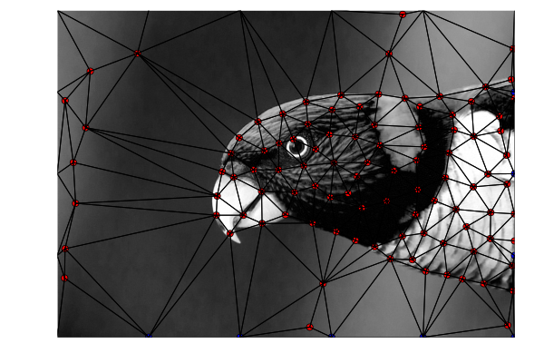
With the workflow more or less working, I ran some profiling to see if I could
speed it up. Unsurprisingly, generating the weighted points was one area where a
lot of time was spent, though it’s not yet clear if that’s because it’s python
code or because that’s genuinely one of the most complex parts of the code – my
best Julia alternative was to write my own short Shannon entropy function and
make it search locally with ImageFiltering::mapwindow

function shannon(w::AbstractMatrix)
   cm = collect(values(countmap(w))) / sum(size(w)) / 256
   sum([-x * log2(x) for x in cm])
end

mapwindow(shannon, image, (19, 19))

though, this creates a square subsampling, whereas the python version uses a nicer disk.

The profiling shows a lot of blank areas, and I’m not sure how to interpret those

Profile’s @profview output in VS Code

I realised at this point that I actually didn’t know how long the python version takes
to run. I grabbed the original source code
and tried running it (after installing the relevant python packages) but it failed –
some packages had changed their arguments and signatures since this was written. A couple
of small updates later, my fork
now runs the code. It doesn’t take terribly long to run – it doesn’t display the image,
it saves it, and I’m not sure if that’s a factor. I (naively?) expected that the Julia
version would be a lot faster, and I’m hopeful that there’s performance I’ve left on the
table.

If anyone is interested in playing with a small-ish Julia package, feel free to poke at
this – it’s definitely not being used for anything critical.

For now, I’m enjoying throwing images at this and getting some nice looking results

If you’re interested in having a play with this package or helping to improve it,
it’s on GitHub – I’m not planning
to publish it to the registry any time soon, but that’s perhaps something to look
forward to in the future. For now, the main issues I see with this package are:

The white border around the produced image remains – I have tried setting
margin=0mm but that doesn’t appear to help
Performance is not as good as it can be, I suspect; the entropy calculation
(calling python) is definitely a bottleneck.
To speed up the processing, only every 10th pixel is used to determine the
average colour of the triangle – this may fail to identify an entire triangle.
CI – I generated this package in VSCode using PkgTemplates and it is the
first Julia package I’ve built. CI failed immediately, so I’ve probably done
something wrong.
I am still somewhat of a beginner in Julia, so there are probably many places
in which improvements can be made – feel free to suggest them!

As always, I can be found on Mastodon and
the comment section below.

devtools::session_info()

“`{r sessionInfo, echo = FALSE}
devtools::session_info()
“`

Working with vectors using DataFrames.jl minilanguage

By: Blog by Bogumił Kamiński

Re-posted from: https://bkamins.github.io/julialang/2024/02/02/combine.html

Introduction

I have written in the past about DataFrames.jl operation specification syntax
(also called minilanguage), see for example this post or this post.

Today I want to discuss one design decision made in this minilanguage and its consequences.
It is related with how vectors are handled when they are returned from some transformation function.

The post was written under Julia 1.10.0 and DataFrames.jl 1.6.1.

A basic example

Consider the following example, where we want to compute a profit from some sales data:

julia> using DataFrames

julia> df = DataFrame(name=["A", "B", "C"],
                      revenue=[10, 20, 30],
                      cost=[5, 12, 18])
3×3 DataFrame
 Row │ name    revenue  cost
     │ String  Int64    Int64
─────┼────────────────────────
   1 │ A            10      5
   2 │ B            20     12
   3 │ C            30     18

julia> combine(df, All(), ["revenue", "cost"] => (-) => "profit")
3×4 DataFrame
 Row │ name    revenue  cost   profit
     │ String  Int64    Int64  Int64
─────┼────────────────────────────────
   1 │ A            10      5       5
   2 │ B            20     12       8
   3 │ C            30     18      12

The crucial point to understand here is that the - function takes
two columns "revenue" and "cost" and returns a vector.
Users typically expect, as in this example, that this vector should
be spread across several rows.

When vector spreading is not desirable?

However, there are cases, when we might not want to spread a vector
into multiple rows. Consider for example a transformation in which
we want to put "revenue" and "profit" values in a 2-element vector
per product. Intuitively we could write something like:

julia> combine(groupby(df, :name),
               All(),
               ["revenue", "cost"] => ((x,y) -> [only(x), only(y)]) => "vec")
ERROR: ArgumentError: all functions must return vectors of the same length

We get an error unfortunately. We will soon understand why, but before
I proceed let me comment on the [only(x), only(y)] part of the definition.
The only function makes sure that we have exactly one row per product.

To diagnose the issue let us drop the All() part in our call:

julia> combine(groupby(df, :name),
               ["revenue", "cost"] => ((x,y) -> [only(x), only(y)]) => "vec")
6×2 DataFrame
 Row │ name    vec
     │ String  Int64
─────┼───────────────
   1 │ A          10
   2 │ A           5
   3 │ B          20
   4 │ B          12
   5 │ C          30
   6 │ C          18

Now we understand the problem. Because our function returns a vector it gets
spread over several rows (which leads to an error as other columns of df have
a different length).

Solving the vector-spreading issue

As I have said above, most of the time vector spreading is a desired feature,
but in the example we have just studied it is not wanted.
For such cases DataFrames.jl allows you to protect vectors from being spread.
What you need to do is to call Ref function on the returned value.
This will protect the result from being spread:

julia> combine(groupby(df, :name),
               All(),
               ["revenue", "cost"] => ((x,y) -> Ref([only(x), only(y)])) => "vec")
3×4 DataFrame
 Row │ name    revenue  cost   vec
     │ String  Int64    Int64  Array…
─────┼──────────────────────────────────
   1 │ A            10      5  [10, 5]
   2 │ B            20     12  [20, 12]
   3 │ C            30     18  [30, 18]

Now, as we wanted, the entries of the "vec" columns are vectors. Wrapping the return
value of our function with Ref protected the vectors from being spread.

The alternative function that you could use to get the same effect is fill:

julia> combine(groupby(df, :name),
               All(),
               ["revenue", "cost"] => ((x,y) -> fill([only(x), only(y)])) => "vec")
3×4 DataFrame
 Row │ name    revenue  cost   vec
     │ String  Int64    Int64  Array…
─────┼──────────────────────────────────
   1 │ A            10      5  [10, 5]
   2 │ B            20     12  [20, 12]
   3 │ C            30     18  [30, 18]

or you could wrap the return value with another pair of [...]:

julia> combine(groupby(df, :name),
               All(),
               ["revenue", "cost"] => ((x,y) -> [[only(x), only(y)]]) => "vec")
3×4 DataFrame
 Row │ name    revenue  cost   vec
     │ String  Int64    Int64  Array…
─────┼──────────────────────────────────
   1 │ A            10      5  [10, 5]
   2 │ B            20     12  [20, 12]
   3 │ C            30     18  [30, 18]

What is going on here? In all three cases (Ref, fill, and [...]) we are wrapping a vector in another object that works like an outer vector.
In the case of [...] it is just a vector, fill produces a 0-dimensional array, and Ref creates a wrapper that behaves like 0-dimensional array.
In all cases DataFrames.jl treats this outer wrapper as a 1-element vector and just stores its contents in a single row (because there is one element to store).

Conclusions

I hope that you will find the example I gave today useful when transforming vectors using DataFrames.jl.

juliabloggers.com

A Julia Language Blog Aggregator