Category Archives: Julia

A multi-language overview on how to document your research project code

By: julia | Victor Boussange

Re-posted from: https://vboussange.github.io/post/documenting-your-research-code/

Documentation serves multiple purposes and may be useful for various audiences, including your future self, collaborators, users and contributors – should you aim at packaging some of your code into a general-purpose library.

This post is part of a series of posts on best practices for managing research project code. Much of this material was developed in collaboration with Mauro Werder as part of the Course On Reproducible Research, Data Pipelines, and Scientific Computing (CORDS). If you have experiences to share or spot any errors, please reach out!

Content

Style guides

The best documentation starts by writing self-explanatory code with good conventions.

Correctly naming your variables enhances code clarity.

There are only two hard things in Computer Science: cache invalidation and naming things.
Martin Fowler

Instead of using generic names like l for a list:

for l in L:
    pass

Use descriptive names like

for line in lines:
    pass

Using style guides for your chosen language ensures consistency and readability in your code. Here are some resources:

Do not hesitate to refactor your code regularly and remove dead code to prevent confusion for yourself and others.

Comments

In-line comments should be used sparingly. Aim to write self-explanatory code instead. Use comments to provide context not apparent from the code itself, such as references to papers, Stack Overflow topics, or TODOs.

Use single-line comments for brief explanations and multi-line comments for more detailed information.

julia

#=
This is a multi-line
comment
=#

python

"""
This is a multi-line
comment
"""

Tip: use vscode rewrap comment/text to nicely format multiline comments.

On top of nicely formatting your code and appending comments where necessary, a literal documentation greatly facilitates the maintenance, understandability and reproducibility of your code.

Literal documentation

Literal documentation helps users understand your tool and get started with it.

README

A README file is essential for any research repository. It is displayed on under the code structure when accessing a GitHub repo.
It should contain:

  • (Badges showing tests, and a nice logo)
  • A one-sentence description of your project
  • A longer description
  • An overview of the repository structure and files
  • Getting started or Examples section
  • An Installation section with dependencies
  • Citation/Reference section
  • (A link to the documentation)
  • (A How to contribute section)
  • An Acknowledgement section
  • License section

Some examples:

API documentation / doc strings

API documentation describes the usage of functions, classes (types) and modules (packages). Parsers usually support markdown styles, which also enhances raw readability for humans. In short, markdown styles consists in using

Doc strings in python live inside the function

def best_function_ever(a_param, another_parameter):
    """
    this is the docstring
    """
    # do some stuff

But above the function or type definition in Julia

"""
this is the docstring
"""
function best_function_ever(a_param, another_parameter)
# do some stuff
end

"Tell whether there are too foo items in the array."
foo(xs::Array) = ...

Best practice for docstrings include

  • (in Julia: insert the signature of your function )
  • Short description
  • Arguments (Args, Input,…)
  • Returns
  • Examples

Several flavours may be used, even for a single language.

python
3 Different documentation style flavours

Google style is easier to read for humans

def add(a, b):
    """
    Add two integers.

    This function takes two integer arguments and returns their sum.

    # Parameters:
    a: The first integer to be added.
    b: The second integer to be added.

    # Return:
    int: The sum of the two integers.

    # Raise:
    TypeError: If either of the arguments is not an integer.

    Examples:
    >>> add(2, 3)
    5
    >>> add(-1, 1)
    0
    >>> add('a', 1)
    Traceback (most recent call last):
        ...
    TypeError: Both arguments must be integers.
    """
    if not isinstance(a, int) or not isinstance(b, int):
        raise TypeError("Both arguments must be integers")
    return a + b

julia

"""
    add(a, b)

Adds two integers.

This function takes two integer arguments and returns their sum.

# Arguments
- `a`: The first integer to be added.
- `b`: The second integer to be added.

# Returns
- The sum of the two integers.

# Examples

```julia-repl
julia> add(2, 3)
5

julia> add(-1, 1)
0
```
"""
function add(a, b)
    return a + b
end

You may use tools like Documenter.jl or Sphinx to automatically render your API documentation on a website. Github actions can automatize the process of building the documentation for you, similarly to how it can automate testing.

Docstrings may be accompanied by typing.

Type annotations

Typing refers to the specification of variable types and function return types within a programming language. It helps define what kind of data a function or variable can handle, ensuring type safety and reducing runtime errors. It

  • clearly indicates the expected input and output types, making the code easier to understand.
  • helps catch type-related errors early in the development process.
  • encourages consistent usage of types throughout the codebase.

python

def add(a: int, b: int) -> int:
    return a + b

In Python, using typing does not enforce type checking at runtime! You may use decorators to enforce it.

julia

function add(a::Int, b::Int)
    return a + b
end

In Julia, types are enforced at runtime! Type annotations help the Julia compiler optimize performance by making type inferences easier.

Consider raising errors

  • We do not like reading manuals. But we are foreced to read error messages. Use assertions and error messages to handle unexpected inputs and guide users.

python

  • assert: When an assert doesn’t pass, it raises an AssertionError. You can optionally add an error message at the end.
  • NotImplementedError, ValueError, NameError: Commonly used, generic errors you can raise. I probably overuse NotImplementedError compared to other types.
def convolve_vectors(vec1, vec2):
    if not isinstance(vec1, list) or not isinstance(vec2, list):
        raise ValueError("Both inputs must be lists.")
    # convolve the vectors

Tutorials

Create tutorial Jupyter notebooks or vignettes in R to demonstrate the usage of your code. Those can be placed in a folder examples or tutorials. Format them as e.g.

  • vignettes in R,
  • or using Jupyter notebooks, which are the perfect format for tutorials

Accessing documentation

julia

?cos
?@time
?r""

python

help(myfun)

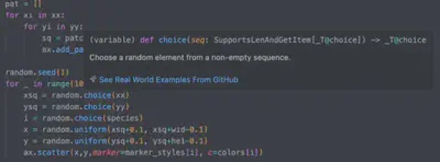
But e.g. VSCode can be also quite helpful, and this works also with your own code!
Doc testing

Doc testing, or doctest, allows you to test your code by running examples embedded in the documentation (docstrings). It compares the output of the examples with the expected results given in the docstrings, ensuring the code works as documented.

Why doc testing?

  • Ensures that the code examples in your documentation are accurate and up-to-date.
  • Simple to write and understand, making it accessible for both writing and reading tests.
  • Promotes writing comprehensive docstrings which enhance code readability and maintainability.

Python

def add(a, b):
    """
    Adds two numbers.

    >>> add(2, 3)
    5
    >>> add(-1, 1)
    0
    """
    return a + b

To run the test:

python -m doctest your_module.py

or from within a script

if __name__ == "__main__":
    import doctest
    doctest.testmod()

julia
Available through Documenter.jl

"""
Adds two numbers.

```jldoctest
julia> add(2, 3)
5

julia> add(-1, 1)
0
```
"""

function add(a, b)
    return a + b
end

Useful packages to help you write and lint your documentation

  • Better Comments

  • Automatic doc string generation

  • Python test explorer

More resources

Take home messages

  • Good documentation helps maintain the long-term memory of a project.
  • Refactor code to reduce complexity instead of documenting tricky code.
  • Writing unit tests is often more productive than extensive documentation.
  • Types of documentation include literal, API, and tutorial/example documentation.
  • Literal documentation explains the big picture and setup.
  • API documentation lives in docstrings and explains function usage.
  • Examples connect the details to common tasks.
  • Consider using tools like ChatGPT to assist with documenting your functions.

Announcing Genie Builder on JuliaHub: Web Apps that Bring your Julia Projects to Life

By: Jasmine Chokshi

Re-posted from: https://info.juliahub.com/blog/announcing-genie-builder-on-juliahub

We are excited to announce the launch of Genie Builder on JuliaHub, a powerful low/no-code tool designed to help you bring your Julia projects to life with beautiful, interactive web applications. Whether you want to build dashboards or complex AI and simulation apps around your Julia code, Genie Builder empowers scientists and developers to create prototypes, internal tools, and even production-grade systems 10x faster and more affordably—all without needing to hire a web development team.

Genie Builder is brought to JuliaHub in partnership with Genie, the leading open-source web framework for Julia. It builds upon Genie’s extensibility and feature-rich foundation, making it an incredibly flexible and robust tool for your web development needs. 

If you have explored some of our Genie resources, then you have seen how Genie Builder accelerates web development with its no-code UI editor helping Julia users with no web development experience to rapidly build complex web apps and dashboards around their code.. Genie Builder builds on Julia’s strengths (high-level, high-performance, dynamic, JIT compiled) so all of your packages and projects can easily be visualized and shared with the world. 

To start, you can learn more about building and deploying apps with Genie Builder and JuliaHub in this webinar.

If you aren’t familiar with how Genie Builder works, here’s the video rundown.

A not so simple coin-tossing game

By: Blog by Bogumił Kamiński

Re-posted from: https://bkamins.github.io/julialang/2024/06/07/probability2.html

Introduction

Two weeks ago I wrote a post about a simple coin tossing game.
Today let me follow up on it with a bit more difficult question and a slightly changed implementation strategy.

The post was written under Julia 1.10.1, DataFrames.jl 1.6.1, and StatsBase.jl 0.34.3.

The problem

Let me describe the setting of a game first (it is similar to what I described in this post).

Assume Alice and Bob toss a fair coin n times. In each toss head (h) or tail (t) can show up with equal probability.

Alice counts the number of times a ht sequence showed.
Bob counts the number of times a hh sequence showed.

The winner of the game is the person who saw a bigger number of occurrences of their favorite sequence.
So for example for n=3. If we get hhh then Bob wins (seeing 2 occurrences of hh, and Alice saw 0 occurrences of ht). If we get hht there is a tie (both patterns ocurred once). If we get tht Alice wins.

The questions are:

  • Who, on the average sees more occurrences of their favorite pattern?
  • Who is more likely to win this game?

Let us try to answer these questions using Julia as usual.

Simulating one game

We start by writing a simulator of a single game:

using Random

function play(n::Integer)
    seq = randstring("ht", n)
    return (hh=count("hh", seq, overlap=true),
            ht=count("ht", seq, overlap=true))
end

The function is not optimized for speed (as we could even avoid storing the whole sequence),
but I think it nicely shows how powerful library functions in Julia are. The randstring function
allows us to generate random strings. In this case consisting of a random sequence of h and t.
Next the count function allows us to count the number of occurrences of desired patterns.
Note that we use the overlap=true keyword argument to count all occurrences of the pattern
(by default only disjoint occurrences are counted).

Let us check the output of a single run of the game:

julia> play(10)
(hh = 3, ht = 3)

In my case (I did not seed the random number generator) we see that for n=10 we got a sequence that
had both 3 occurrences of hh and ht, so it is a tie.

Testing the properties of the game

Here is a simulator that, for a given n, runs the game reps times and aggregates the results:

using DataFrames
using Statistics
using StatsBase

function sim_play(n::Integer, reps::Integer)
    df = DataFrame([play(n) for _ in 1:reps])
    df.winner = cmp.(df.hh, df.ht)
    agg = combine(df,
                  ["hh", "ht"] .=> [mean std skewness],
                  "winner" .=>
                  [x -> mean(==(i), x) for i in -1:1] .=>
                  ["ht_win", "tie", "hh_win"])
    return insertcols!(agg, 1, "n" => n)
end

What we do in the code is as follows. First we run the game reps times and transform a result into a DataFrame.
Next we add a column denoting the winner of the game. In the "winner" column 1 means that hh won, 0 means a tie, and -1 means that ht won.
Finally we compute the following aggregates (using transformation minilanguage; if you do not have much experience with it you can have a look at this post):

  • mean, standard deviation, and skewness of hh and ht counts;
  • probability that ht wins, that there is a tie and that hh wins.

Here is the result of running the code for reps=1_000_000 and n varying from 2 to 16:

julia> Random.seed!(1234);

julia> reduce(vcat, [sim_play(n, 1_000_000) for n in 2:16])
15×10 DataFrame
 Row │ n      hh_mean   ht_mean   hh_std    ht_std    hh_skewness  ht_skewness   ht_win    tie       hh_win
     │ Int64  Float64   Float64   Float64   Float64   Float64      Float64       Float64   Float64   Float64
─────┼────────────────────────────────────────────────────────────────────────────────────────────────────────
   1 │     2  0.25068   0.249825  0.433405  0.432912     1.15052    1.15578      0.249825  0.499495  0.25068
   2 │     3  0.499893  0.499595  0.706871  0.5          1.06068    0.00162      0.374385  0.375765  0.24985
   3 │     4  0.751224  0.748855  0.902063  0.559496     1.0232     0.00312512   0.373833  0.37559   0.250577
   4 │     5  1.00168   1.00012   1.06192   0.612535     0.940274  -6.5033e-5    0.406445  0.28037   0.313185
   5 │     6  1.25098   1.2493    1.19926   0.661162     0.869559  -0.0012833    0.437276  0.233841  0.328883
   6 │     7  1.49972   1.50011   1.32213   0.707523     0.812272  -0.00190003   0.437774  0.234531  0.327695
   7 │     8  1.75064   1.74802   1.43616   0.750169     0.76024    0.00319491   0.440714  0.211252  0.348034
   8 │     9  1.99906   2.00108   1.53902   0.789413     0.715722   0.000107041  0.451749  0.189353  0.358898
   9 │    10  2.24857   2.25009   1.63787   0.829086     0.676735  -0.00207707   0.45343   0.184585  0.361985
  10 │    11  2.50092   2.50007   1.73343   0.867326     0.646397   0.000650687  0.454418  0.175059  0.370523
  11 │    12  2.74753   2.75065   1.81994   0.901478     0.621238  -0.00118389   0.458332  0.164575  0.377093
  12 │    13  2.99635   3.00128   1.90199   0.935108     0.597227   0.00212776   0.460248  0.159239  0.380513
  13 │    14  3.2469    3.25101   1.9814    0.96887      0.575535  -0.000255108  0.460817  0.154523  0.38466
  14 │    15  3.50074   3.49934   2.05981   0.998945     0.55527    0.000827465  0.461547  0.147699  0.390754
  15 │    16  3.75258   3.7513    2.13521   1.03027      0.538056   0.000772964  0.463627  0.142931  0.393442

What do we learn from these results?

On the average hh and ht occur the same number of times.
We see this from "hh_mean" and "ht_mean" columns.
This is expected. As in a given sequence of two observations hh and ht have the same
probability of occurrence (0.25) the result just follows the linearity of expected value.
We can see that as we increase n the values in these columns increase roughly by 0.25.

However, the probability of ht winning is higher than the probability of hh winning
(except n=2 when it is equal). We can see this from the "ht_win" and "hh_win" columns.
This is surprising as the patterns occur, on the average the same number of times.

To understand the phenomenon we can look at the "hh_std", "ht_std",
"hh_skewness", and "ht_skewness" columns.
We can clearly see that hh pattern count has a higher standard deviation and for n>2 it is positively skewed
(while ht has zero skewness).
This means that hh counts are more spread (i.e. they can be high, but also low).
Additionally we have few quite high values balanced by more low values for hh relatively to ht (as the means for both patterns are the same). This, in turn, means that if hh wins over ht then it wins by a larger margin, but it happens less rarely than seeing ht winning over hh.

The core reason for this behavior was discussed in my previous post. The hh values can cluster (as e.g. in the hhh pattern), while ht patterns cannot overlap.

Conclusions

I hope you found this puzzle interesting. If you are interested how the properties we described can be proven analytically I recommend you check out this paper.