By: Tamás K. Papp

Re-posted from: https://tamaspapp.eu/post/common-random-variables/

Motivation

When simulating models with random components, it is frequently advantageous to decompose the structure into

1. parameters \(\theta\) that we need to characterize structural relationships,

2. noise \(\varepsilon\) that is independent of parameters,

3. a function \(f(\theta, \varepsilon)\) that generates observed data or moments.

Doing this allows us to use common random variables (aka common random numbers), which is a technique which simply keeps \(\varepsilon\) fixed for different \(\theta\). This can help with making \(f\) differentiable, which allows the use of derivative-based optimization algorithms (eg for maximum likelihood or MAP) or derivative-based MCMC methods. It is also used to reduce the variance of simulated moments.

When implementing this technique in Julia, I frequently create a wrapper structure that saves the \(\varepsilon\), allocating an Array which can be updated in place. Since a redesign of DynamicHMC.jl is coming up which will accommodate simulated likelihood methods in a more disciplined manner, and I wanted to explore other options, most importantly StaticArrays.jl.

Here I benchmark the alternatives for Julia v0.6.2 using a simple toy model. TL;DR for the impatient: StaticArrays.jl is 150x faster, and this does not depend on using immutable or mutable StaticArrays, or even reallocating every time new \(\varepsilon\)s are generated.

Problem setup

The setup is simple: we draw \(M\) observations, and our noise is

\[
\varepsilon_{i,j} \sim N(0, 1)
\qquad
\text{for } i = 1, \dots, M; j = 1, \dots, 7.
\]

Our parameters are \(\mu\) and \(\sigma\), and for each \(i\) we calculate

\[
A_i = \frac17 \sum_{j=1}^7 \exp(\mu + \sigma \varepsilon_{i,j})
\]

which is the sample average after a nonlinear transformation. The \(7\) is a bit accidental, it comes from simplifying an actual problem I am working on. We are interested in the sample average for \(A_i\). I deliberately refrain micro-optimizing each version, to reflect how I would approach a real-life problem.

We code the common interface as

using BenchmarkTools
using StaticArrays
using Parameters

# common interface

"Dimension of noise ``ϵ`` for each observation."
const EDIM = 7

"""
Common random variables. The user needs to define

1. `observation_moments`, which should use `observation_moment`,
2. `newcrv = update!(crv)`, which returns new common random variables,
potentially (but not necessarily) overwriting `crv`.
"""
abstract type CRVContainer end

observation_moment(ϵ, μ, σ) = mean(@. exp(μ + σ * ϵ))

average_moment(crv::CRVContainer, μ, σ) = mean(observation_moments(crv, μ, σ))

"Calculate statistics, making `N` draws, updating every `L`th time."
function stats(crv, μ, σ, N, L)
    _stat() = (N % L == 0 && (crv = update!(crv)); average_moment(crv, μ, σ))
    [_stat() for _ in 1:N]
end

The way I wrote stats is representative of how I use HMC/NUTS: simulated moments on the same trajectory are calculated with the same \(\varepsilon\)s, which are updated for each trajectory. Of course, the parameters would change along the trajectory; here they don’t, but this does not affect the benchmarks.

The semantics of update! allows both in-place modifications and a functional style.

Using a preallocated matrix

This is the standard way I would write this.¹ \(\varepsilon\)s are in columns of a matrix, which is preferable for mapping them as slices, then they are mapped using observation_moment.

update! overwrites the contents.

"""
Common random variables are stored in columns of a matrix.
"""
struct PreallocatedMatrix{T} <: CRVContainer
    ϵ::Matrix{T}
end

PreallocatedMatrix(M::Int) = PreallocatedMatrix(randn(EDIM, M))

update!(p::PreallocatedMatrix) = (randn!(p.ϵ); p)

observation_moments(p::PreallocatedMatrix, μ, σ) =
    vec(mapslices(ϵ -> observation_moment(ϵ, μ, σ), p.ϵ, 1))

Using static vectors

We share the following between various static vector implementations:

"Common random variables as a vector of vectors, in the `ϵs`."
abstract type CRVVectors <: CRVContainer end

observation_moments(p::CRVVectors, μ, σ) =
    map(ϵ -> observation_moment(ϵ, μ, σ), p.ϵs)

I find the use of map more intuitive here than mapslices above.

Static vectors, container preallocated

In the first version using static vectors, we keep SVector in a Vector, and update in place.

struct PreallocatedStaticCRV{K, T} <: CRVVectors
    ϵs::Vector{SVector{K, T}}
end

PreallocatedStaticCRV(M::Int) =
    PreallocatedStaticCRV([@SVector(randn(EDIM)) for _ in 1:M])

function update!(p::PreallocatedStaticCRV)
    @unpack ϵs = p
    @inbounds for i in indices(ϵs, 1)
        ϵs[i] = @SVector(randn(EDIM))
    end
    p
end

Mutable static vectors, overwritten

We modify this to use mutable vectors — this should not make a difference.

struct MutableStaticCRV{K, T} <: CRVVectors
    ϵs::Vector{MVector{K, T}}
end

MutableStaticCRV(M::Int) =
    MutableStaticCRV([@MVector(randn(EDIM)) for _ in 1:M])

function update!(p::MutableStaticCRV)
    @unpack ϵs = p
    @inbounds for i in indices(ϵs, 1)
        randn!(ϵs[i])
    end
    p
end

Static vectors, allocated each time

Finally, for the third solution,

struct GeneratedStaticCRV{K, T} <: CRVVectors
    ϵs::Vector{SVector{K, T}}
end

GeneratedStaticCRV(M::Int) =
    GeneratedStaticCRV([@SVector(randn(EDIM)) for _ in 1:M])

update!(p::GeneratedStaticCRV{K, T}) where {K, T} =
    GeneratedStaticCRV([@SVector(randn(T, K)) for _ in indices(p.ϵs, 1)])

Results

Running

@btime mean(stats(PreallocatedMatrix(100), 1.0, 0.1, 100, 10))
@btime mean(stats(PreallocatedStaticCRV(100), 1.0, 0.1, 100, 10))
@btime mean(stats(MutableStaticCRV(100), 1.0, 0.1, 100, 10))
@btime mean(stats(GeneratedStaticCRV(100), 1.0, 0.1, 100, 10))

we obtain

As a preview of future improvements, I tried PreallocatedMatrix on current master (which will become Julia v0.7, obtaining 3.5 ms (2.46 MiB), which is really promising.²

The conclusion is that StaticArrays simplifies and speeds up my code at the same time. I especially like the last version (GeneratedStaticCRV), because it obviates the need to think about types in advance. While here the example is simple, in practice I would use automatic differentiation, which makes it more challenging to determine buffer types in advance. I expect I will transition to a more “buffer-free” style in the future, and design the interface for DynamicHMC.jl accordingly.

PS: From now on, my blog posts with Julia code will have a banner about version information.

By: Mosè Giordano

Re-posted from: http://giordano.github.io/blog/2018-03-22-astroimages/

In the last days I worked on a very little
package: AstroImages.jl.
Written in the Julia programming language and part of
the JuliaAstro organization, this package
provides simple tools to visualize astronomical images saved
in FITS files.

AstroImages.jl is meant as an interface to popular Julia packages
like Images.jl
and Plots.jl, and
uses FITSIO.jl to read FITS files.

Currently the package supports only single-frame images, in gray scale.

AstroImages.jl is licensed under the MIT “Expat” License.

Installation

The package is available for Julia 0.6 but not yet registered, thus if you would
like to try it out use the following command in the Julia REPL:

julia> Pkg.clone("https://github.com/JuliaAstro/AstroImages.jl")

Usage

After installing the package, you can start using it with

julia> using AstroImages

For the time being the package provides only two functions:

• load (extending the load function
  from FileIO.jl), to load an
  extension of a FITS file
• AstroImage, a type constructor to create a new astronomical image object.

Reading extensions from FITS file

You can load and read the the first extension of a FITS file with load:

julia> load("file.fits")
1300×1200 Array{UInt16,2}:
[...]

The second, optional, argument of this load method is the number of the
extension to read. Read the third extension of the file with:

julia> load("file.fits", 3)
1300×1200 Array{UInt16,2}:
[...]

AstroImage type

The package provides a new type, AstroImage to integrate FITS images with
Julia packages for plotting and image processing. The AstroImage function has
the same syntax as load. This command:

julia> img = AstroImage("file.fits")
AstroImages.AstroImage{UInt16,ColorTypes.Gray}[...]

will read the first extension from the file.fits.

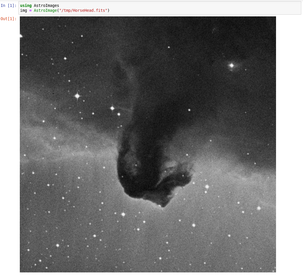
If you are working in a Jupyter notebook, an
AstroImage object is automatically rendered as a PNG image:

Plotting an AstroImage

An AstroImage object can be plotted with the Plots.jl package. Just use

julia> using Plots

julia> plot(img)

and the image will be displayed as a heatmap using your favorite backend.

Feedback welcome

If you test the package and would like to suggest improvements, feel free to
file an issue on GitHub or, even better, send a pull request to add new features
yourself!