Keno Fischer, Julia Computing Co-Founder and Chief Technology Officer (Tools) participated in a Quora Session March 18-23. What are the biggest software challenges in machine learning and…

By: Dean Markwick's Blog -- Julia

Re-posted from: https://dm13450.github.io/2019/04/10/Turing-Sampling-Speed.html

The Turing.jl package provides a great interface
for performing Bayesian inference using a variety of algorithms. But
what algorithm allows you to go from data to samples the quickest? In
this blog post I will be sampling from a simple model to demonstrate
how quickly you can sample from a model. This is useful
for anyone that has a Turing model in the middle of another model that
they need to get samples from.

Toy Model

For the toy model we will be sampling from the Beta distribution.

using Distributions

testData = rand(Beta(3, 4), 100);

Writing the model in Julia is simple enough. We will be using an
inverse Gamma prior for the free parameters.

using Turing
Turing.turnprogress(false)

@model betaSample(y) = begin
    
    alpha ~ InverseGamma(2, 1/8)
    beta ~ InverseGamma(2, 1/8)
    
    for i in eachindex(y)
        y[i] ~ Beta(alpha, beta)
    end
	end
	
sample(betaSample(testData), MH(250))

[MH] Finished with
  Running time        = 0.6196572280000009;
  Accept rate         = 0.028;

Object of type Chains, with data of type 250×4×1 Array{Union{Missing, Float64},3}

Log evidence      = 0.0
Iterations        = 1:250
Thinning interval = 1
Chains            = 1
Samples per chain = 250
internals         = elapsed, lp
parameters        = alpha, beta

parameters
       Mean    SD   Naive SE  MCSE    ESS 
alpha 0.4483 0.1063   0.0067 0.0453 5.4955
 beta 0.2394 0.0461   0.0029 0.0191 5.8285

This quick test verifies that I’ve written the model correctly and everything can be sampled.

Available Samplers

In this blog post I am interested in being able to quickly sample from the posterior distribution and extract some sensible parameter samples. I will be assessing 4 different samplers.

• Hamiltonian Monte Carlo (HMC)
• Metropolis Hastings (MH)
• No U Turn Sampling (NUTS)
• Stochastic Gradient Langevin Dynamics (SGLD)

Each have their own way of sampling from the posterior distribution,
with benefits and drawbacks. Turing provides an standard interface to
use these algorithms without having to worry about the fine details.

We want to be able to ‘set and forget’ the parameters of the sampler
so will be using the defaults given at
http://turing.ml/docs/sampler-viz/. If the sampling fails, I will
tweak the parameters until it works.

I’ve chosen these 4 samplers out of familiarity. HMC and NUTS are the
algorithms used in Stan. Metropolis Hastings is the one sampler
everyone has implemented themselves at one point and SGLD is an
improved version of that. I’m not including the particle samplers,
mainly because I’m unfamiliar with their use cases.

We will be running the samplers for 1000 iterations and benchmarking for 120 seconds. This should give us enough trials to calculate an average running time of the samplers.

using BenchmarkTools
BenchmarkTools.DEFAULT_PARAMETERS.seconds = 120.0

numIts = 1000

HMC

hmcSamps = sample(betaSample(testData), HMC(numIts, 0.01, 10));
hmcRunTime = @benchmark sample(betaSample($testData), HMC($numIts, 0.01, 10));

Metropolis Hastings

mhSamps = sample(betaSample(testData), MH(numIts));
mhRunTime = @benchmark sample(betaSample($testData), MH($numIts));

NUTS

nutsSamps = sample(betaSample(testData), NUTS(numIts, 0.65));
nutsRunTime = @benchmark sample(betaSample($testData), NUTS($numIts, 0.65));

SGLD

sgldSamps = sample(betaSample(testData), SGLD(numIts, 0.01));
sgldRunTime = @benchmark sample(betaSample($testData), SGLD($numIts, 0.01));

Results

using Plots

function extractMeanTime(runtime)
    median(runtime).time /1e9 
end

nms = ["SGLD", "HMC", "MH", "NUTS"]
runTimes = [sgldRunTime, hmcRunTime, mhRunTime, nutsRunTime]

times = map(extractMeanTime, runTimes)

map(length, runTimes)

4-element Array{Int64,1}:
 340
  38
 287
  23

Here we can see that each sampler has been evaluated a number of times. The median running time is extracted and converted into seconds.

bar(nms, times, ylabel="Average Time (seconds)", legend=false)

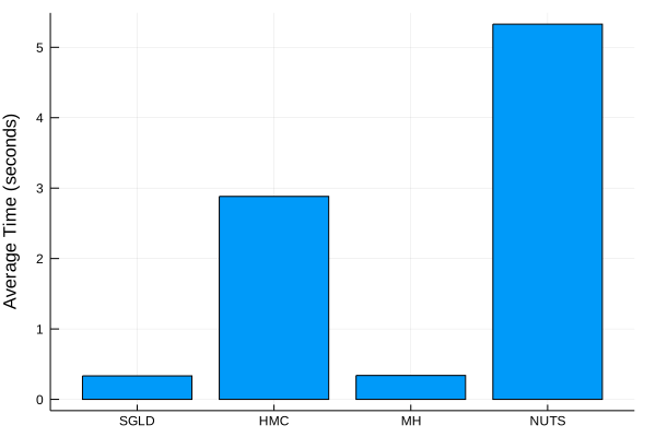
HMC and NUTS are the slowest. SGLD and MH performing the
quickest which is the expected result. The calculations involved in
the HMC and NUTS algorithms are a bit more complex.

However, it is not always about speed. We want to make sure that the
sampler is moving towards the correct parameters and not just moving
about randomly. We need to a check the quality of the samples. To assess this we want to check the Effective Number
of Samples which is a metric that discounts the samples by the
autocorrelation between values. Essentially, a better sampling
algorithm will produce a higher number of effective samples for the
same number of iterations.

Therefore, instead of just looking at the running time, we want to
divide the effective sample size by the running time to produce a
Effective Samples per Second value.

function extractMeanandESS(smps)
    params = MCMCChains.summarystats(smps)
    alphaESS = params.summaries[1].value[1, 5,1]
    betaESS = params.summaries[1].value[2, 5,1]
    
    alphaMean = params.summaries[1].value[1, 1,1]
    betaMean = params.summaries[1].value[2, 1,1]
    
    [alphaMean, betaMean, alphaESS, betaESS]
end

allSamps = [sgldSamps, hmcSamps, mhSamps, nutsSamps]
params = map(extractMeanandESS, allSamps)
paramSummaries = reduce(hcat, params)'

4×4 LinearAlgebra.Adjoint{Float64,Array{Float64,2}}:
 2.6097  3.1185   22.4958   21.1824
 2.8535  3.3886  424.781   458.39  
 0.3993  0.7389   11.0827    9.3238
 2.9507  3.5326   51.6685   39.9213

using StatsPlots
alphaESSperSecond = paramSummaries[:,3] ./ times
betaESSperSecond = paramSummaries[:,4] ./ times

groupedbar(nms, hcat(alphaESSperSecond, betaESSperSecond), label=["Alpha", "Beta"], ylabel="Effective Samples per Second")

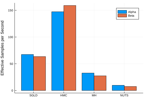
So NUTS produces the least amount of effective samples per second run. Which is surprising, but for such a simple model it doesn’t cause too much of a concern. I would predict that as the model increased in complexity, the ESS would improve compared to the other samplers.

From this graph, we are inclined to think that either HMC or SGLD are the preferable sampling algorithms.

Parameter Results

pdfs = map(x-> pdf.(Beta(x[1], x[2]), collect(0:0.01:1)), params)

histogram(testData, normed=true, label="Training Data", fillalpha=0.4)

plot!(collect(0:0.01:1), pdfs[1], label=nms[1], linewidth=2)
plot!(collect(0:0.01:1), pdfs[2], label=nms[2], linewidth=2)
plot!(collect(0:0.01:1), pdfs[3], label=nms[3], linewidth=2)
plot!(collect(0:0.01:1), pdfs[4], label=nms[4], linewidth=2)
plot!(collect(0:0.01:1), pdf.(Beta(3,4), collect(0:0.01:1)), label="True", linewidth=2)

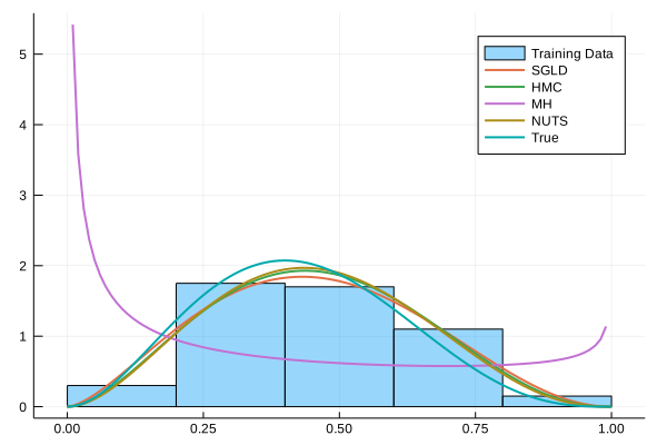
Here we can see that the Metropolis Hastings sampler is nowhere near the true distribution. All the others have done well and are close to the true distribution. Given that they only have 100 datapoints to go by and we are just taking the mean of the samples its not a bad result.

Conclusion

So in conclusion it looks like we would be inclined to use the HMC
sampler. It produces the best ESS per second values and doesn’t
require too much tinkering with. If speed is an absolute priority,
then SGLD might be more appropriate, its 6 times faster at the cost of
about 100 effective samples a second.

Definitely do not use Metropolis Hastings though. Out of the box it hasn’t even got close to the correct value. I’m probably missing setting some parameter.

There are a number of weaknesses in this analysis. Firstly, we have not considered multiple chains to check for convergence. Currently, multiple chains in parallel are not supported out of the box for Turing.jl so rather than faff about using multiple chains by hand, I’ve just stuck to the one. Secondly, BenchmarkTools runs for a fixed amount of time rather than a fixed amount of samples. I’ve changed the parameters of the benchmark to try and account for this, but it still isn’t exact.
Finally, there are still the particle samplers. I’ve shied away from
them, mainly because I’ve never used them before and not 100% on their
use case.

Keno Fischer, Julia Computing Co-Founder and Chief Technology Officer (Tools) participated in a Quora Session March 18-23.

What will machine learning look like 15-20 years from now?

Machine learning is a very rapidly moving field, so it’s hard to make predictions about the state of the art 6 months from now, let alone 15 – 20 years. I can however, offer a series of educated guesses based on what I see happening right now.

1. We are still far away from AGI. Current generation machine learning systems are still very far away from something that could legitimately be called artificial “intelligence”. The systems we have right now are phenomenal at pattern recognition from lots of data (even reinforcement learning systems are mostly about memorizing and recognizing patterns that worked well during training). This is certainly a necessary step, but it is very far away from an intelligent system. In analogy to human cognition, what we have now is analogous to the subconscious processes that allow split second activation of your sympathetic nervous system when your peripheral vision detects a predator approaching or a former significant other turning around a corner – in other words, pattern-based, semi-automatic decisions that our brain does “in hardware”. We don’t currently have anything I can see that would resemble intentional thought and I’m not convinced we’ll get to it from current generation systems.

2. Traditional programming is not going away. I sometimes hear the claim that most traditional programming will be replaced by machine learning systems. I am highly skeptical of this claim, partly as a corollary to the previous point, but more generally because machine learning isn’t required for the vast majority of tasks. Machine learning excels where dealing with the messiness of the real world, lots of data is available and no reasonably fundamental model is available. If any of these are not true, you generally don’t have to settle for a machine learning model – the traditional alternatives are superior. A fun way to think about it is that humans are the most advanced natural general intelligence around, but yet we invented computers to do certain specialized tasks we’re too slow at. Why should we expect artificial intelligence to be any different?

3. Machine learning will augment most traditional tasks. That being said, any time one of these traditional systems needs to interact with a human, there is an opportunity for machine-learning based augmentation. For example, a programmer looking at error messages could use a machine learning system that looks at the error messages and suggests a course of action. Computers are a lot more patient than humans. You can’t make a human watch millions of hours of programming sessions to remember the common resolutions to problems, but you can make a machine learning system do the same. In addition, machine learning systems can learn from massive amounts of data very rapidly and on a global scale. If any instance of the machine learning system has ever encountered a particular set of circumstances, it can almost instantly share that knowledge globally, without being limited to the speed of human communication. I don’t think we have yet begun to appreciate the impact of this, but we’ll probably see it in another 5-10 years.

4. We’ll get better at learning from small or noisy data. At the moment, machine learning systems mostly require large amounts of relatively clean, curated, data sets. There are various promising approaches to relax this requirement in one or the other direction (or combinations of small, well curated data sets to get started with a larger corpus of more noisy data). I expect these to be perfected in the near future.

5. We’ll see ML systems be combined with traditional approaches. At the moment it seems fairly common to see ML systems that are entirely made of neural networks trying to solve end to end problems. This often works ok, because you can recover many traditional signal processing techniques from these building blocks (e.g. Fourier transforms, edge detection, segmentation, etc.), but the learned versions of these transforms can be significantly more computationally expensive than the underlying approach. I wouldn’t be surprised to see these primitives making a bit of a comeback (as part of a neural network architecture). Similarly, I’m very excited about physics-based ML approaches where you combine a neural network with knowledge of an underlying physical model (e.g. the differential equations governing a certain process) in order to outperform both pure ML approaches and approaches relying solely on the physical process (i.e. simulations).