Category Archives: Julia

Generated constant propagation; hold on to your britches!

By: Jacob Quinn

Re-posted from: https://quinnj.home.blog/2019/06/20/generated-constant-propagation-hold-on-to-your-britches/

In a recent JuliaLang Discourse post, OP was looking for a simple way to convert their Vector{CustomType} to a DataFrame, treating each CustomType element as a “row”, with the fields of CustomType as fields in the row. The post piqued my interest, given my work on the Tables.jl interface over the last year. Tables.jl is geared specifically towards creating generic access patterns to “table” like sources, specifically providing Tables.rows and Tables.columns as two ways to access table data from any source. Tables.columns returns a “property-accessible object” of iterators, while Tables.rows returns the dual: an iterator of “property-accessible objects” (property-accessible object here is defined as any object that supports both propertynames(obj) and getproperty(obj, prop), which includes all custom structs by default).

I decided to respond by showing how simple it can be to “hook in” to the Tables.jl world of interop; my code looked like:

using DataFrames, Random, Tables

struct Mine
a::Int
b::Float64
c::Matrix{Float64}
end

Tables.istable(::Type{Vector{Mine}}) = true
Tables.rowaccess(::Type{Vector{Mine}}) = true
Tables.rows(x::Vector{Mine}) = x
Tables.schema(x::Vector{Mine}) = Tables.Schema((:a, :b), Tuple{Int, Float64})

Random.seed!(999)
v = [Mine(rand(1:10), rand(), rand(2,2)) for i ∈ 1:10^6];
df = DataFrame(v)

But when doing a quick benchmark of the conversion from Vector{Mine} to DataFrame, it was 3x-5x slower than other methods already proposed. Huh? I started digging. One thing I noticed was by ***not*** defining Tables.schema, the code was a bit faster! That led me to assume something was up in our schema-based row-to-column code.

Part of the challenge with this functionality is wrestling with providing a fast, type-stable method for building up strongly-typed columns for a set of rows with arbitrary number of columns and types. Just iterating over a row in a for-loop, accessing each field programmatically can be disastrous; because each extracted field value in the hot for-loop could be a number of types, the compiler can’t do much more than create a Core.Box to put arbitrary values in, then pull out again for inserting into the vector we’re building up. Yuck, yuck, yuck; if you see Core.Boxs in your @code_typed output, or values inferred as Any, it’s an indication the compiler just couldn’t figure out anything more specific, and in a hot for-loop called over and over and over again, any hope of performance is toast.

Enter meta-programming: Tables.jl tries to judiciously employ the use of @generated functions to help deal w/ the issue here. Specifically, when doing this rows-to-columns conversion, with a known schema, Tables.eachcolumn can take the column names/types as input, and generate a custom function with this aforementioned “hot for-loop” unrolled. That is, instead of:

for rownumber = 1:number_of_rows
row = rows[rownumber]
for i = 1:ncols
column[i][rownumber] = getfield(row, i)
end

end

For a specific table input’s schema, the generated code looks like:

for rownumber = 1:number_of_rows
row = rows[rownumber]
column[1][rownumber] = getfield(row, 1)
column[2][rownumber] = getfield(row, 2)
# etc.
end

What makes this code ***really*** powerful is the compiler’s ability to do “constant propagation”, which means that, while compiling, when it encounters getfield(row, 1), it can realize, “hey, I know that row is a Mine type, and I see that they’re calling getfield to get the 1 field, and I happen to know that the 1 field of Mine is an Int64, so I’ll throw that information into dataflow analysis so things can get further inlined/optimized”. It’s really the difference between the scenario I described before of the compiler just having to treat the naive for-loop values as Any vs. recognizing that it can figure out the exact types to expect which can make the operation we’re talking about here boil down to a very simple “load”, then “store”, without needing to box/unbox or rely on runtime dynamic dispatch based on types.

Back to the original issue: why was this code slower than the unknown schema case? Well, it turns out that our generated code was actually trying to be clever by calculating a run-length encoding of consecutive types for a schema, then generating mini type-stable for-loops; i.e. the generated code looked like:

for rownumber = 1:number_of_rows
row = rows[rownumber]
# if columns 1 & 2 are Int64
for col = 1:2
column[col][rownumber] = getfield(row, col)
end
# column 3 is a Float64
for col = 3:3
column[col][rownumber] = getfield(row, col)
end
# columns 4 & 5 are Int64 again
for col = 4:5
column[col][rownumber] = getfield(row, col)
end
# etc.
end

While this is clever, and can generate less code when schema types tend to be “sticky” (i.e. lots of the same type consecutively), the problem is in the getfield(row, col) call. Even though the call to each getfield ***should*** be type-stable, as calculated from our run-length encoding, the compiler unfortunately can’t figure that out inside these mini type-stable for-loops. This means no super-inlining/optimizations, so things end up being slower.

So what’s the conclusion here? What can be done? The answer was pretty simple, instead of trying to be extra clever with run-length encodings, if the schema is small enough, just generate the getfield calls directly for each column. The current heuristic is for schemas with less than 100 columns, the code will be generated directly, and for larger schema cases, we’ll try the run-length encoding approach (since it’s still more efficient than the initial naive approach).

Hope you enjoyed a little dive under the hood of Tables.jl and some of the challenges the data ecosystem faces in the powerful type system of Julia. Ping me on twitter with any thoughts or questions.

Cheers.
Deep Learning: Exploring High Level APIs of Knet.jl and Flux.jl in comparison to Tensorflow-Keras

By: Estadistika -- Julia

Re-posted from: https://estadistika.github.io//julia/python/packages/knet/flux/tensorflow/machine-learning/deep-learning/2019/06/20/Deep-Learning-Exploring-High-Level-APIs-of-Knet.jl-and-Flux.jl-in-comparison-to-Tensorflow-Keras.html

When it comes to complex modeling, specifically in the field of deep learning, the go-to tool for most researchers is the Google’s TensorFlow. There are a number of good reason as to why, one of it is the fact that it provides both high and low level APIs that suit the needs of both beginners and advanced users, respectively. I have used it in some of my projects, and indeed it was powerful enough for the task. This is also due to the fact that TensorFlow is one of the most actively developed deep learning framework, with Bayesian inference or probabilistic reasoning as the recent extension (see TensorFlow Probability, another extension is the TensorFlow.js). While the library is written majority in C++ for optimization, the main API is served in Python for ease of use. This design works around the static computational graph that needs to be defined declaratively before executed. The static nature of this graph, however, led to difficulty on debugging the models since the codes are itself data for defining the computational graph. Hence, you cannot use a debugger to check the results of the models line by line. Thankfully, it’s 2019 already and we have a stable Eager Execution that allows users to immediately check the results of any TensorFlow operations. Indeed, this is more intuitive and more pythonic. In this article, however, we’ll attempt to explore, what else we have in 2019. In particular, let’s take look at Julia’s deep learning libraries and compare it to high level APIs of TensorFlow, i.e. Keras’ model specification.

As a language that leans towards numerical computation, it’s no surprise that Julia offers a number of choices for doing deep learning, here are the stable libraries:

  1. Flux.jl – The Elegant Machine Learning Stack.
  2. Knet.jl – Koç University deep learning framework.
  3. MLJ.jl – Julia machine learning framework by Alan Turing Institute.
  4. MXNet.jl – Apache MXNet Julia package.
  5. TensorFlow.jl – A Julia wrapper for TensorFlow.

Other related packages are maintained in JuliaML. For this article, we are going to focus on the usage of
Flux.jl and Knet.jl, and we are going to use the Iris dataset for classification task using Multilayer Perceptron. To start with, we need to install the following packages. I’m using Julia 1.1.0. and Python 3.7.3.


Loading and Partitioning the Data

The Iris dataset is available in the RDatasets.jl Julia package and in Python’s Scikit-Learn. The following codes load the libraries and the data itself.


The random seed set above is meant for reproducibility as it will give us the same random initial values for model training. The iris variable in line 11 (referring to Julia code) contains the data, and is a data frame with 150 × 5 dimensions, where the columns are: Sepal Length, Sepal Width, Petal Length, Petal Width, and Species. There are several ways to partition this data into training and testing datasets, one procedure is to do stratified sampling, with simple random sampling without replacement as the sampling selection within each stratum — the species. The following codes define the function for partitioning the data with the mentioned sampling design:


Extract the training and testing datasets using the function above as follows:


All three codes above extract xtrn, the training data (feature) matrix of size 105 × 4 (105 observations by 4 features) dimensions; ytrn, the corresponding training target variable with 105 × 1 dimension; xtst, the feature matrix for testing dataset with 45 × 4 dimensions; and ytst, the target variable with 45 × 1 dimension for testing dataset. Moreover, contrary to TensorFlow-Keras, Knet.jl and Flux.jl need further data preparation from the above partitions. In particular, Knet.jl takes minibatch object as input data for model training, while Flux.jl needs one-hot encoding for the target variables ytrn and ytst. Further, unlike Knet.jl which ships with minibatch function, Flux.jl gives the user the flexibility to create their own.

Specify the Model

The model that we are going to use is a Multilayer Perceptron with the following architecture: 4 neurons for the input layer, 10 neurons for the hidden layer, and 3 neurons for the output layer. The first two layers contain bias, and the neurons of the last two layers are activated with Rectified Linear Unit (ReLU) and softmax functions, respectively. The diagram below illustrates the architecture described:


The codes below specify the model:


Coming from TensorFlow-Keras, Flux.jl provides Keras-like API for model specification, with Flux.Chain as the counterpart for Keras’ Sequential. This is different from Knet.jl where the highest level API you can get are the nuts and bolts for constructing the layers. Having said, however, Flux.Dense is defined almost exactly as the Dense struct of the Knet.jl code above (check the source code here). In addition, since both Flux.jl and Knet.jl are written purely in Julia, makes the source codes under the hood accessible to beginners. Thus, giving the user a full understanding of not just the code, but also the math. Check the screenshots below for the distribution of the file types in the Github repos of the three frameworks:


From the above figure, it’s clear that Flux.jl is 100% Julia. On the other hand, Knet.jl while not apparent is actually 100% Julia as well. The 41.4% of Jupyter Notebooks and other small percentages account for the tutorials, tests and examples and not the source codes.


Train the Model

Finally, train the model as follows for 100 epochs:


The codes (referring to Julia codes) above save both loss and accuracy for every epoch into a data frame and then into a CSV file. These will be used for visualization. Moreover, unlike Flux.jl and Knet.jl which require minibatch preparation prior to training, TensorFlow-Keras specifies this on fit method as shown above. Further, it is also possible to train the model in Knet.jl using a single function without saving the metrics. This is done as follows:


The Flux.jl code above simply illustrates the use of Flux.@epochs macro for looping instead of the for loop. The loss of the model for 100 epochs is visualized below across frameworks:

From the above figure, one can observe that Flux.jl had a bad starting values set by the random seed earlier, good thing Adam drives the gradient vector rapidly to the global minimum. The figure was plotted using Gadfly.jl. Install this package using Pkg as described in the first code block, along with Cario.jl and Fontconfig.jl. The latter two packages are used to save the plot in PNG format, see the code below to reproduce:

Evaluate the Model

The output of the model ends with a vector of three neurons. The index or location of the neurons in this vector defines the corresponding integer encoding, with 1st index as setosa, 2nd as versicolor, and 3rd as virginica. Thus, the codes below take the argmax of the vector to get the integer encoding for evaluation.


The figure below shows the traces of the accuracy during training:

TensorFlow took 25 epochs before surpassing 50% again. To reproduce the figure, run the following codes (make sure to load Gadfly.jl and other related libraries mentioned earlier in generating the loss plots):

Benchmark

At this point, we are going to record the training time of each framework.


The benchmark was done by running the above code repeatedly for about 10 times for each framework, I then took the lowest timestamp out of the results. In addition, before running the code for each framework, I keep a fresh start of my machine.

The code of the above figure is given below (make sure to load Gadfly.jl and other related libraries mentioned earlier in generating the loss plots):

Conclusion

In conclusion, I would say Julia is worth investing even for deep learning as illustrated in this article. The two frameworks, Flux.jl and Knet.jl, provide a clean API that introduces a new way of defining models, as opposed to the object-oriented approach of the TensorFlow-Keras. One thing to emphasize on this is the for loop which I plainly added in training the model just to save the accuracy and loss metrics. The for loop did not compromise the speed (though Knet.jl is much faster without it). This is crucial since it let’s the user spend more on solving the problem and less on optimizing the code. Further, between the two Julia frameworks, I find Knet.jl to be Julia + little-else, as described by Professor Deniz Yuret (the main developer), since there are no special APIs for Dense, Chains, etc., you have to code it. Although this is also possible for Flux.jl, but Knet.jl don’t have these out-of-the-box, it ships only with the nuts and bolts, and that’s the highest level APIs the user gets. Having said, I think Flux.jl is a better recommendation for beginners coming from TensorFlow-Keras. This is not to say that Knet.jl is hard, it’s not if you know Julia already. In addition, I do love the extent of flexibility on Knet.jl by default which I think is best for advanced users. Lastly, just like the different extensions of TensorFlow, Flux.jl is flexible enough that it works well with Turing.jl for doing Bayesian deep learning, which is a good alternative for TensorFlow Probability. For Neural Differential Equations, Flux.jl works well with DifferentialEquations.jl, checkout DiffEqFlux.jl.

Next Steps

In my next article, we will explore the low level APIs of Flux.jl and Knet.jl in comparison to the low level APIs of TensorFlow. One thing that’s missing also from the above exercise is the use of GPU for model training, and I hope to tackle this in future articles. Finally, I plan to test these Julia libraries on real deep learning problems, such as computer vision and natural language processing (checkout the workshop on these from JuliaCon 2018).

Complete Codes

If you are impatient, here are the complete codes excluding the benchmarks and the plots. These should work after installing the required libraries shown above:


References

Software Versions

Tricksy Tuple Types…

By: Jacob Quinn

Re-posted from: https://quinnj.home.blog/2019/06/19/tricksy-tuple-types/

Some of you may be aware of my obsession with JSON libraries, and it’s true, there’s something about simple data formats that sends my brain into endless brainstorming of ways to optimize reading, writing, and object-mapping in the Julia language. JSON3.jl is my latest attempt at a couple of new ideas for JSON <=> Julia fun. The package is almost ready for a public release, and I promise I’ll talk through some of the fun ideas going on there, but today, just wanted to point out a tricky performance issue that took a bit of sleuthing to track down.

Here’s the scenario: we have a string of JSON like {"a": 1}, super simple right? In the standard Julia JSON.jl library, you just call JSON.parse(str) and get back a Dict{String, Any}. In JSON3.jl, we have a similar “plain parse” option which looks like JSON3.read(str), which returns a custom JSON3.Object type which I can talk about in another post in more detail. Another option in JSON3.jl, is to do JSON3.read(str, Dict{String, Any}), i.e. we can specify the type we’d like to parse from any string of JSON. While doing some quick benchmarking to make sure things look reasonable, I noticed JSON3.jl was about 2x slower compared to both JSON.parse, and JSON3.read(str, Dict{String, Int}). Hmmm, what’s going on here??

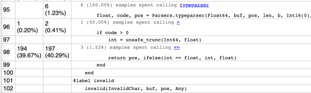
I first turned to profiling, and used the wonderful StatProfilerHTML.jl package to inspect my profiling results. That’s when I noticed around ~40% of the time was spent on a seemingly simple line of code:

Hmmmm……a return statement with a simple ifelse call? Seems fishy. Luckily, there’s a fun little project called Cthulhu.jl, which allows debugger “stepping” functionality with Julia’s unparalleled code inspection tools (@code_lowered, @code_typed, @code_llvm, etc.). As I “descended into madness” to take a look at the @code_typed of this line of code, I found this:

%1865 = (JSON3.ifelse)(%1864, %1857, %1851)::Union{Float64, Int64}
%1866 = (Core.tuple)(%1853, %1865)::Tuple{Int64,Union{Float64, Int64}}

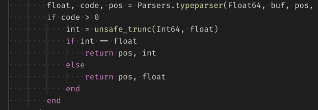
Ruh-roh Shaggy…….the issue here is this Tuple{Int64,Union{Float64,Int64}} return type. It’s not concrete and leads to worse type inference in later code that tries to access this tuple’s second element. This is also undesirable because we know that the value should be either an Int64 or Float64, so ideally we could structure things so that code generation can just do a single branch and generate nice clean code the rest of the way down. If we change the code to:

Let’s take another cthulic descent and check out the generated code:

%1863 = (%1857 === %1862)::Bool
│ │ @ float.jl:484 within `==' @ float.jl:482
│ │┌ @ bool.jl:40 within `&'
│ ││ %1864 = (Base.and_int)(%1861, %1863)::Bool
│ └└
└──── goto #691 if not %1864
@ /Users/jacobquinn/.julia/dev/JSON3/src/structs.jl:330 within `read' @ /Users/jacobquinn/.julia/dev/JSON3/src/structs.jl:99
690 ─ %1866 = (Core.tuple)(%1853, %1857)::Tuple{Int64,Int64}
└──── goto #693
@ /Users/jacobquinn/.julia/dev/JSON3/src/structs.jl:330 within `read' @ /Users/jacobquinn/.julia/dev/JSON3/src/structs.jl:101
691 ─ %1868 = (Core.tuple)(%1853, %1851)::Tuple{Int64,Float64}
└──── goto #693

Ah, much better! Though there’s a few more steps, we can now see we’re getting what we’re after: our return type will be Tuple{Int64,Int64} or Tuple{Int64,Float64} instead of Tuple{Int64,Union{Int64,Float64}}. And the final performance results? Faster than JSON.jl!

Thanks for reading and I’ll try to get things polished up in JSON3.jl soon so you can take it for a spin.

Feel free to follow me on twitter, ask questions, or discuss this post there ?

Cheers.