Category Archives: Julia

Building a constraint programming solver in Julia

More than 2 years ago I wrote a Sudoku solver in Python. I really enjoyed it and therefore I’ve spend some time to do the same in Julia just faster 😉 Then I wanted to build a whole constraint-programming solver in Julia. Well I actually still want to do it. It will be hard but fun. I want to share my way on my blog and instead of writing when I’ve done something I want to share my journey while I’m doing it.

Additionally the blog should be as simple as possible and everyone should be able to follow step by step.

In my dream we are building this together so if there is someone out there who is crazy and wants to build a constraint-programming solver from scratch… Send me a mail ([email protected]) and/or comment on this post.

In this first post I’ll create the package and create test cases as well as building the most basic solver using backtracking. In the next stages we will build the alldifferent, straights, sum constraint and so on together. The next post will be similar to the previous Sudoku post but with animation and of course written in Julia.

Let’s get started:

First we create a package:

julia
(v1.2) pkg> generate ConstraintSolver
Generating project ConstraintSolver:
    ConstraintSolver/Project.toml
    ConstraintSolver/src/ConstraintSolver.jl

(v1.2) pkg> activate ConstraintSolver/
Activating environment at `~/Julia/ConstraintSolver/Project.toml`

(v1.2) pkg> develop .
 Resolving package versions...
  Updating `~/.julia/environments/v1.2/Project.toml`
  [e0e52ebd] + ConstraintSolver v0.1.0 [`../../../Julia/ConstraintSolver`]
  Updating `~/.julia/environments/v1.2/Manifest.toml`
  [e0e52ebd] + ConstraintSolver v0.1.0 [`../../../Julia/ConstraintSolver`]

Info: You get to the package mode with ].

I want to have a git repository for the project and we can do this inside the julia shell as well.

shell> cd ConstraintSolver/
/home/ole/Julia/ConstraintSolver

shell> git init
Initialized empty Git repository in /home/ole/Julia/ConstraintSolver/.git/

Info: You get to the shell mode with ;.

The next thing for me is always to create a simple test file which I call current.jl which is inside .gitignore so that I can test the same thing on different branches.

shell> mkdir test
shell> touch test/current.jl
shell> vim .gitignore

Now before we do something like loading modules I would advise to use Revise which helps in general to avoid reloading the REPL when we change code.

julia> using Revise

The current.jl file is not a real test it’s more like a playground.

Inside I wrote:

using ConstraintSolver

CS = ConstraintSolver
include("sudoku_fcts.jl")

function main()
    com = CS.init()

    grid = zeros(Int8,(9,9))
    grid[1,:] = [0 0 0 5 4 6 0 0 9]
    grid[2,:] = [0 2 0 0 0 0 0 0 7]
    grid[3,:] = [0 0 3 9 0 0 0 0 4]
    grid[4,:] = [9 0 5 0 0 0 0 7 0]
    grid[5,:] = [7 0 0 0 0 0 0 2 0]
    grid[6,:] = [0 0 0 0 9 3 0 0 0]
    grid[7,:] = [0 5 6 0 0 8 0 0 0]
    grid[8,:] = [0 1 0 0 3 9 0 0 0]
    grid[9,:] = [0 0 0 0 0 0 8 0...

When do micro-optimizations matter in scientific computing?

By: Christopher Rackauckas

Re-posted from: http://www.stochasticlifestyle.com/when-do-micro-optimizations-matter-in-scientific-computing/

Something that has been bothering me about discussions about microbenchmarks is that people seem to ignore that the benchmarks are highly application-dependent. The easiest way to judge whether the benchmark really matters to a particular application is the operation overhead of the largest and most common calls. If you have a single operation dominating all of your runtime 99.9%, making everything else 100x faster still won’t do anything to your real runtime performance. But at the same time, if your bottleneck is some small operation that’s in a tight loop, then that operation may be your bottleneck. This is a classic chart to keep in the back of your mind when considering optimizations.

Here is a very brief overview on what to think about when optimizing code and how to figure out when to stop.

Function Call Overhead

When dealing with scalar operations, the cost of basic operations matters a lot. And one basic operation that can bite you in higher level languages is the function call overhead. Notice that 10’s of basic arithmetic (more with SIMD) can happen in the time that a single function can be called. Slower languages, like Python and R, have a higher function call overhead than something like C++, Fortran, of Julia for a few reasons. First of all it’s calling the function dynamically so there’s a lookup involved (and in Julia, if types are unstable there is a lookup as well, this is the cost of a “dynamic dispatch”). But secondly, in these compiled languages, of a function is determined to be sufficiently cheap, the function call can be completely gotten rid of by inlining the function (this is essentially copy-pasting the code in, instead of making it call the function). The heuristics for deciding whether a function is costly enough to inline is then very in-depth, since inlining a function means that a separately compiled function cannot be called so it’s a trade-off between run-time and compile-time speed. If the function costs too much, then inlining essentially is not helpful so you’d prefer to just compile faster, while if the function is cheap then it’s necessary to inline since otherwise the dominating cost is the function call.

In some domains this matters a lot. Ordinary differential equations for example are defined by huge swaths of scalar operations (this is one example of a common stiff ODE benchmark). If you had high operation overhead there your performance would be destroyed, which is why this domain has not only traditionally been dominated by compiled languages, but this domain is still dominated by compiled languages (counting Julia as one). In domains like optimization, ODEs, and nonlinear solving, this is particularly an issue for interpreted languages because these mathematical problems are higher order functions. This means that the API requires a function that is defined by the user, but the repeated calls to the interpreted function is the mostly costly part of the calculation, and so performance can be very hurt in this scenario. Even when accelerators like Numba are used, the context switch between the interpreted and compiled code can still hurt performance. The only way around this of course is to make an interface where you never accept a function from the user and instead you build it for them. This is why Pyomo is a Python optimization library where you use a modeling object. In both cases, a compiled function is built behind the scenes so that no interpreters get in the way.

But as you go up in computational cost per function, the performance lost by the function overhead cost goes down. This is why in languages like Python or R vectorization is encouraged because the 350ns or so function call cost is then dominated by the cost of the function calculation itself (and the cost is high enough that inlining doesn’t even play into the picture). Just for comparison, that’s taking scalar operations like + and * from 5ns-20ns to 350ns… so now you know where that performance went. With C++, Fortran, or Julia, it doesn’t matter whether you vectorize or loop through scalar operations because the vectorized call and the loop are the same under the hood, dropping down to optimally low function call cost or inlining it to remove the cost entirely (whereas the interpreted vectorized call is essentially the same as the compiled loop).

When do heap allocations matter?

Another major issue that comes up is heap allocations. The idea in brief is, allocations have a high floor and scale ~O(n). Let’s demonstrate this with some vectorized functions. First, let’s do element-wise multiplication.

using LinearAlgebra, BenchmarkTools
function alloc_timer(n)
    A = rand(n,n)
    B = rand(n,n)
    C = rand(n,n)
    t1 = @belapsed $A .* $B
    t2 = @belapsed ($C .= $A .* $B)
    t1,t2
end
ns = 2 .^ (2:11)
res = [alloc_timer(n) for n in ns]
alloc   = [x[1] for x in res]
noalloc = [x[2] for x in res]
 
using Plots
plot(ns,alloc,label="=",xscale=:log10,yscale=:log10,legend=:bottomright,
     title="Micro-optimizations matter for BLAS1")
plot!(ns,noalloc,label=".=")
savefig("microopts_blas1.png")

In this case we see that there’s almost a 3x-5x across the board advantage (remember the graph is log-scale) to using allocation-free interfaces because the allocation of the output array scales with the size of the array, and it has a high overhead. However, when we get to matrix multiplications, the scaling of the calculation comes into play:

using LinearAlgebra, BenchmarkTools
function alloc_timer(n)
    A = rand(n,n)
    B = rand(n,n)
    C = rand(n,n)
    t1 = @belapsed $A*$B
    t2 = @belapsed mul!($C,$A,$B)
    t1,t2
end
ns = 2 .^ (2:9)
res = [alloc_timer(n) for n in ns]
alloc   = [x[1] for x in res]
noalloc = [x[2] for x in res]
 
using Plots
plot(ns,alloc,label="*",xscale=:log10,yscale=:log10,legend=:bottomright,
     title="Micro-optimizations only matter for small matmuls")
plot!(ns,noalloc,label="mul!")
savefig("microopts.png")

Notice that when the matrix multiplications are small, the non-allocating `mul!` form has an advantage because of the high overhead of an allocation. However, as the size of the matrices increase, the O(n^3) scaling of matrix multiplication becomes the dominant force, and so the cost of the allocation is negligible.

Optimizing Machine Learning and Partial Differential Equations

So how much do different disciplines require lower level features? It turns out that same aspects of technical computing really require fast function calls and scalar operations, like solving nonlinear differential equations, and thus something like C++, Fortran, or Julia is really required for top notch speeds. In other disciplines, the time is completely dominated by large matrix multiplication or convolutional kernels. Machine learning is a prime example of this, where >99% of the computation time is spent inside of the large matrix multiplication of dense layers or convolution calls of a convolutional neural network. For these functions, pretty much every language, (R, Python, Julia, MATLAB, Octave, etc.), is calling into a BLAS implementation. One popular one is OpenBLAS, while another is Intel’s MKL. When things move to the GPU, essentially everyone is calling NVIDIA’s CuBLAS and cuDNN. With large matrix operations taking on the order of minutes (to even hours as it gets large and distributed), the 350ns function call overhead of a slow language just doesn’t even matter anymore.

The same tends to happen with PDE solving, where the dominant costs are sparse matrix multiplications and sparse factorizations, usually handled by SuiteSparse or libraries like PETSc when you start to get parallel. Here, factorizations taking an hour isn’t even uncommon, so I think you could sparse a few milliseconds. At this point, what matters more than a micro-optimization is the strategy that is used: whoever uses the last matrix multiplications or matrix factorizations wins the game.

This doesn’t mean that the underlying libraries can be written in a slow language. No, these pieces, like SuiteSparse, OpenBLAS, etc. need to be in a fast language like C++ or Fortran (or even Julia is starting to see performant BLAS implementations). But calling and using libraries in this domain tends to have negligible overhead.

I will just end by noting that big data analysis with pre-written kernels is another area that falls into this performance domain, while the moment you allow users to write their own kernels (“give me a function and I’ll do a map reduce with it!”) you suddenly need to compile that function in a fast way.

Optimizing Scientific Machine Learning and Differentiable Programming

When you get to scientific machine learning and differentiable programming, things get tricky. If you haven’t heard of scientific machine learning, read this overview of the tools of the domain, and for differentiable programming this paper is a good overview of things people (we) are trying to target with the technique. The amount of micro-optimizations that you need really depends on where you fall in this spectrum from numerical ODEs to machine learning. Generally, if your matrices are “small enough”, you need to use mutation and make sure scalar usage is fast, while once the matrices are large enough then all of the time is taken in GPU BLAS kernels so the name of the game is to use a better strategy.

There is a minor caveat here because tracing-based ADs, like Flux’s Tracker, PyTorch, or TensorFlow Eager, have a really really high op overhead. PyTorch announced that its overhead cost has gotten to 1us. Again, when matrix multiplications are clearly larger than seconds or minutes in any machine learning task, this overhead is so low that it does not make an impact on the total time itself, so we should congratulate the machine learning libraries for essentially eliminating overhead for their standard use case. But remember that if you compare that to the 5ns-20ns of basic scalar cost for things like `+` and `*`, you can see that, for example, tracing-based reverse mode automatic differentiation through the definition of a nonlinear ordinary differential equation will be horrifyingly slow. This means that tracing-based ADs do not do well in more general-purpose codes, making it difficult to use for things like differentiable programming in scientific machine learning where neural networks are mixed with large nonlinear kernels.

There is a way through though. Zygote has showcased operation overheads of around 500ns. The way this is done is through source-to-source automatic differentiation. This isn’t new, and the very old ADIFOR Fortran AD was a source-to-source AD that first noticed major per-op overhead advantages. The reason is because a tracing-based reverse-mode AD needs to build a tape at every single step so that way it knows the operations and the values. This tape needs to be heap allocated in any sensibly large calculation. This is why x[1] + x[2]*x[3] turns into a whopping multi-microsecond calculation when being traced while only being a ~20ns fma call if just scalar! A source-to-source AD doesn’t need to build a trace because it has already built and compiled an entire adjoint code. It does need to still store some values (since values from the forward pass need to be used in the backpass), and there are multiple ways that one can go about doing this. Zygote heap allocates forward values by making closures, this is where most of its overhead seems to come from. ADIFOR mixes forward mode in when it needs to compute values, which is another valid strategy. There are ways to also precompute some values of the fly while going in reverse, or mixing different strategies such as checkpointing. I think there’s a lot that can done to better optimize reverse-mode ADs like Zygote for the case of scalar operations (in fact, there seem to be quite a few compiler optimizations that it’s currently missing), and so if you plan to reverse-mode a bunch of scalar codes this may be an area of study to track in more detail.

Conclusion

The art of optimizing code is to only optimize what you need to. If you have small function calls (such as having lots of scalar operations), use a fast language and tools with low operation overhead. If you have really costly operations, then it really doesn’t matter what you do: optimize the costly operations. If you don’t know what regime your code lives in… then profile it. And remember that allocation costs scale almost linearly, so don’t worry about them if you’re doing O(n^3) operations with large n. You can use these ideas to know if using a feature from a higher level language like Python or R is perfectly fine performance-wise for the application. That said, this is also a good explanation as to why the libraries for those languages are not developed within the language and instead drop down to something else.

The post When do micro-optimizations matter in scientific computing? appeared first on Stochastic Lifestyle.

ANN: DynamicHMC 2.0

By: TamĂĄs K. Papp

Re-posted from: https://tamaspapp.eu/post/2019-08-29-dynamichmc2/

I am very pleased to announce version 2.0 of DynamicHMC.jl. I briefly summarize the new the developments in this blog post.

Code used in this post was written for Julia v1.* and, when applicable, reflects the state of packages used on 2019-09-03. You may need to modify it for different versions.

Note: my blog no longer has a comment section. Feel free to ask questions about this post on the Julia Discourse forum.

Some context

DynamicHMC.jl is part of a collection of packages for implementing Bayesian inference using a modular approach:

  1. TransformVariables.jl just maps \(\mathbb{R}^n\) vectors into collections of constrained parameters, like positive real numbers or valid correlation matrices,

  2. LogDensityProblems.jl provides an interface for log density functions \(\mathbb{R}^n \to \mathbb{R}\) and their derivative, also calculating the latter using automatic differentiation via one of the supported native Julia AD frameworks (see below),

  3. DynamicHMC.jl, which just takes a log density and its gradient on \(\mathbb{R}^n\), and performs MCMC using NUTS,

  4. MCMCDiagnostics.jl for generic convergence diagnostics (ie not specific to a particular MCMC method).

In contrast to a single interface and a DSL for describing models, these packages provide a suite of tools for modern MCMC, with easily interchangable and modular building blocks. For example, the gradients of a log density can be obtained with

  1. ForwardDiff.jl, which is very robust,
  2. ReverseDiff.jl, which works better for medium-sized problems using a classic taped approach,
  3. Flux.jl which is more modern and can be faster on larger problems, and of course
  4. Zygote.jl which is very promising, but work in progress;

and switching between these usually just requires changing a single line. I find this especially important since as Zygote keeps maturing, it will play a more and more important role for fast AD. Moreover, the user is free to code all gradients manually, or just parts of them to help out AD, for example with the adjoint method.

In addition to this, some packages use DynamicHMC.jl as a backend. This is encouraged and remains to be supported. Finally, the third common use case for this package is as a research platform for experimenting with modern HMC algorithms: this is supported by a detailed documentation of internals.

Why a new API was needed

As bug reports and test cases kept accumulating, it was very clear that better adaptation heuristics, and a more sophisticated diagnosic and warmup interface was needed. When NUTS/HMC goes wrong with models it should be able to handle otherwise, the problem is usually with adaptation. The user should be able to learn what went wrong, and either manually tune stepsize and the kinetic energy metric, or choose an adaptation better suited to the model.

The old API of DynamicHMC was lacking in several ways. The main entry point was something like

chain, tuning = NUTS_init_tune_mcmc(∇P, 1000)

with tuning containing the adapted stepsize and kinetic energy metric.

In practice, it turns out that

  1. either the model works fine, and then the user cares little about warmup,
  2. or it doesn’t, then information about the warmup would be necessary to debug the model.

Fine-tuning the adaptation sequence was possible, but rather unintuitive in the old API. I doubt that many people used this feature, or were even aware that it was available. Statistics on why adaptation failed or sampling didn’t mix were also difficult to obtain.

After collecting the various problems, I spent some time on redesigning the internals, then the API to address all major issues.

Here I would like to thank all users of this library who provided a lot of valuable feedback, especially in the form of bug reports which I could study and use to tweak the sampler. Robert J Goedman coded all the models of the excellent “Statistical Rethinking” book in DynamicHMCModels.jl, which is the most comprehensive collection of examples for this package, and also provides and extremely useful test suite for it. DiffEqBayes.jl included DynamicHMC as a backend, while Soss.jl provides a higher-level DSL for building models. Users (who are, mostly, also the authors) of these packages provided a lot of example models and test cases.

Changes in 2.0

Documentation

The documentation was rewritten from scratch, now including a worked example. All functions of the API have extensive docstrings, usually with examples where relevant. This documentation should be the starting point for using this package.

Of course, if you have questions, feature requests, or bug reports, don’t hesitate to open an issue; I would like to emphasize that it is still perfectly fine to open issues just to ask questions. You can also address questions to @Tamas_Papp on the Julia discourse forum.

Main interface

Most people would now call the sampler with

results = mcmc_with_warmup(Random.GLOBAL_RNG, ∇P, 1000)

where ∇P is an object that supports the LogDensityProblems.jl API (basically “give me a log density and its gradient at this position”, withs some bells and whistles). results is a NamedTuple with fields like chain (a vector of positions in \(\mathbb{R}^n\), which most users probably need to transform into a collection of constrained parameters), information on tree statistics and the adapted parameters. A detailed worked example is available.

In contrast to the previous API, the random number generator needs to be explicitly provided. This is in preparation for multithreading, encouraging the user to be conscious of RNGs as mutable states; the internals now also follow this approach with no default RNG in the sampling part.

Exposed warmup building blocks

The new API allows fine-grained control over the warmup stages. For example, this is how one would skip local optimization, ask for a dense (Symmetric) metric instead of the default Diagonal, and provide an initial position while at the same time allowing the stepsize to be found and adapted using the default heuristic:

q = ... # some initial position
warmup_stages = default_warmup_stages(; local_optimization = nothing,
                                      M = Symmetric)
Îș = GaussianKineticEnergy(5, 0.1)
mcmc_with_warmup(rng, ℓ, N;
                 initialization = (q = q, Îș = Îș),
                 warmup_stages = warmup_stages)

The warmup_stages above is just a Tuple, with no secret sauce, you are provided the tools to make up your own if necessary.

Changed heuristics and warmup defaults

In contrast to Stan, the old API did not look for a local optimum before starting the stepsize adaptation. This is fine in most cases, but occasionally adapting to an otherwise atypical region of the parameter space can cause problems with the algorithm later on. On the other hand, adapting too eagerly to models with singularities in the log posterior can also backfire very easily.

The new default heuristics make a half-hearted effort to go near some local optimum, but don’t overdo it, which I think is the right compromise. Also, there is some protection against singularities on the “edges” of \(\mathbb{R}^n\) (which can happen with the “funnels” of hierarchical models).

Stepsize adaptation became a bit more robust with some tweaks. I still think that the initial bracketing algorithm in this package is better than Stan’s in some cases and worth the extra couple of evaluations, as it plays nicer with the dual averaging for posteriors where the optimal stepsize can change rapidly.

The default kinetic energy metric is now Diagonal. This should be nearly optimal except for very heavily correlated posteriors which also happen to be devoid of any other pathologies (this is rare in practice).

Diagnostics

Diagnostics were reorganized into a DynamicHMC.Diagnostics submodule of their own. They are intended for interactive use, and the exposed API can change with just a minor version increment. You can import them into your current module with

using DynamicHMC.Diagnostics

Note that this package has no plotting functionality. Use your favorite plotting package to visualize information, I made the plots below with PGFPlotsX.jl (and relevant code may eventually end up in a mini-package, for now see the link below).

download code as plots.jl

Detailed tree statistics

Each result that contains a chain also comes with corresponding tree_statistics, which is a vector of statistics for each NUTS step. It contains information about acceptance ratios, number of leapfrog steps and tree depth, and the doubling directions. In 2.0, it also contains a field which informs the user about the location (in steps relative to the starting point).

There is a summarize_tree_statistics function that produces a useful summary about acceptance rations:

julia> results = mcmc_with_warmup(Random.GLOBAL_RNG, ℓ, 1000;
                                  reporter = NoProgressReport());

julia> results.tree_statistics[1]
DynamicHMC.TreeStatisticsNUTS(-1.7246438302263802, 2,
                              turning at positions 1:4, 0.963443025058039,
                              7, DynamicHMC.Directions(0x595b1b9c))

julia> summarize_tree_statistics(results.tree_statistics)
Hamiltonian Monte Carlo sample of length 1000
  acceptance rate mean: 0.94, 5/25/50/75/95%: 0.75 0.92 0.97 1.0 1.0
  termination: divergence => 0%, max_depth => 0%, turning => 100%
  depth: 0 => 0%, 1 => 14%, 2 => 55%, 3 => 21%, 4 => 10%, 5 => 0%

Calculating leapfrog trajectories

A call not unlike

traj = leapfrog_trajectory(ℓ, [0, -2], 0.2, -6:10;
                           Îș = GaussianKineticEnergy(2),
                           p = [2, 2])

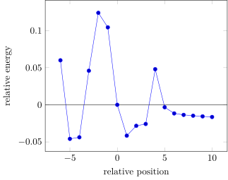
was used to produce the information that was used for the plot below. The resulting vector (here, traj) contains a NamedTuple of positions, momenta, and relative energy. Here the stepsize \(\epsilon = 0.2\) was selected to on purpose as near-but-not-quite-unstable, starting from position [0, -2], taking 6 leapfrog steps backward and 10 forward.
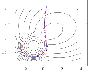
Hamiltonian trajectory

The plot below visualizes the energy relative to the starting point.
Relative energy

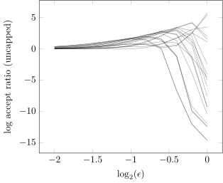
Exploring log acceptance ratios

It can be very useful to explore log acceptance ratios. explore_log_acceptance_ratios returns a matrix of them with random momenta. In the plot below, we can see things become iffy for \(\epsilon > 0.5\), approximately.
Internal changes

Although there is a new API, the bulk of the changes were internal: resulting in (hopefully) much cleaner and more generic code, better unit tests, and improved documentation documentation for the internals, which are especially relevant for users using this package for research. If this affects you, please read the code and the docstrings and feel free to ask questions.