By: Tom Kwong's Infinite Loop

Re-posted from: https://ahsmart.com/pub/programming-is-boring-art/index.html

Programming is boring art

Read more

By: Dean Markwick's Blog -- Julia

Re-posted from: https://dm13450.github.io/2020/05/26/HawkesProcessesPackage.html

HawkesProcesses.jl is a Julia package that provides a number of
functions to model events using a Hawkes process. This vignette
demonstrates how you can use the package and fit Hawkes processes to
your data. Here are the fine details on the
Hawkes process maths.

So download the package and you can follow along with my post.

using HawkesProcesses
using Distributions
using Plots

Enjoy these types of posts? Then sign up for my newsletter.

Intensity of a Hawkes Process

bg = 0.5
kappa = 0.5
kernel(x) = pdf.(Distributions.Exponential(1/0.5), x)
maxT = 100;

We calculate the intensity of a Hawkes process with default parameters all equal to 0.5 between 0 and 10 with two events at t = 3 and 6.

ts = 0:0.1:10
testEvents = [3, 6]
intensity = HawkesProcesses.intensity(collect(ts), testEvents, bg, kappa, kernel);

plot(ts, intensity, xlabel = "Time", ylabel = "Intensity", label="")

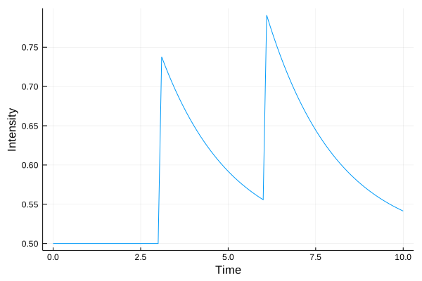
As expected two spikes of intensity when the events occur.

Simulating a Hawkes Process

simevents = HawkesProcesses.simulate(bg, kappa, kernel, maxT);

We now simulate events with default parameters from t=0 to t=100.

ts = collect(0:0.1:maxT)
intensity = HawkesProcesses.intensity(ts, simevents, bg, kappa, kernel)
plot(ts, intensity, xlabel="Time", ylabel = "Intensity", label="")
plot!(simevents, repeat([mean(intensity)], length(simevents)), seriestype=:scatter, label="Events")

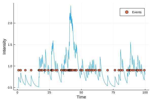
Again, spikes of events occurring followed by slightly quieter periods which shows the clustering effect of the Hawkes process.

Bayesian Estimation of a Hawkes Processs using a Latent Variable

This package provides an enhanced method of MCMC sampling of the Hawkes process parameters. By exploiting a latent variable (mathematical details can be found here) we are able to more efficiently sample from the posterior distribution than by doing direct Gibbs sampling using the likelihood and prior.

bg = 0.5
kappa = 0.5
kernel(x) = pdf.(Distributions.Exponential(1/0.5), x)
maxT = 1000
simevents = HawkesProcesses.simulate(bg, kappa, kernel, maxT);

bgSamps, kappaSamps, kernSamps = HawkesProcesses.fit(simevents, maxT, 1000);

plot(histogram(bgSamps, label="Background", colour=:darkred), 
    histogram(kappaSamps, label="Kappa", colour=:darkblue), 
    histogram(kernSamps, label="Kernel", colour=:darkgreen), layout = (1, 3))

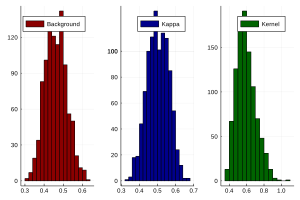
The histograms of the parameter samples are distributed around the true values as expected which shows our method is working. We run another chain to check convergence.

bgSamps2, kappaSamps2, kernSamps2 = HawkesProcesses.fit(simevents, maxT, 1000);

bgplot = plot(bgSamps, label="Chain 1", title="Background")
bgplot = plot!(bgplot, bgSamps2, label="Chain 2")

kappaplot = plot(kappaSamps, label="Chain 1", title="Kappa")
kappaplot = plot!(kappaSamps2, label="Chain 2")

kernplot = plot(kernSamps, label="Chain 1", title="Kernel")
kernplot = plot!(kernSamps2, label="Chain 2")

plot(bgplot, kappaplot, kernplot, layout = (1, 3))

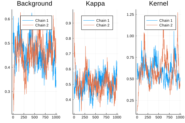
A basic visual inspection shows that the chains are exploring the parameter space nicely.

Hawkes Process Likelihood

The likelihood of a Hawkes process can be used in a number of ways. It can assess the goodness of fit of a particular parameter set or it can be used to estimate parameters aswell.

bg = 0.5
kappa = 0.5
kernelDist =  Distributions.Exponential(1/0.5)
kernel_f(x) = pdf.(kernelDist, x)
maxT = 1000
simevents = HawkesProcesses.simulate(bg, kappa, kernel_f, maxT);

trueLikelihood = HawkesProcesses.likelihood(simevents, bg, kappa, kernelDist, maxT)

-963.4283337185043

bgArray = collect(0.1:0.05:1)
bgLikelihood = map(x -> HawkesProcesses.likelihood(simevents, x, kappa, kernelDist, maxT), bgArray)
bgPlot = plot(bgArray, bgLikelihood, xlabel="Parameter Values", ylabel = "Likelihood", label="Background", colour=:darkred);

kappaArray = collect(0.1:0.05:1)
kappaLikelihood = map(x -> HawkesProcesses.likelihood(simevents, bg, x, kernelDist, maxT), kappaArray)
kappaPlot = plot(kappaArray, kappaLikelihood, xlabel="Parameter Values", ylabel = "Likelihood", label="Kappa", colour=:darkblue);

kernArray = collect(0.01:0.01:1)
kernLikelihood = map(x -> HawkesProcesses.likelihood(simevents, bg, kappa, Distributions.Exponential(1/x), maxT), kernArray)
kernPlot = plot(kernArray, kernLikelihood, xlabel="Parameter Values", ylabel = "Likelihood", label="Kernel", colour=:darkgreen);

plot(bgPlot, kappaPlot, kernPlot, layout=(3,1))

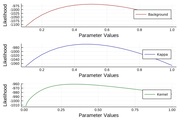
Here we demonstrate the shape of the likelihood for the different values in parameters. As expected the likelihood reaches its maximum value at the true values.

Maximum Likelihood Estimation of a Hawkes Process

Using the likelihood function from HawkesProcesses we can use optimisation to find the parameters that produce the maximum values of the likelihood.

using Optim
function exp_mle(params, events, maxT)
    if any(params .< 0)
        return Inf
    end
    
    bg = params[1]
    kappa = params[2]
    kernParam = params[3]
    
    -1*HawkesProcesses.likelihood(events, bg, kappa, Distributions.Exponential(kernParam), maxT)
end

opt = optimize(x->exp_mle(x, simEvents, maxT), rand(3)*10)
Optim.minimizer(opt)

3-element Array{Float64,1}:
 0.5155810722101667 
 0.47205389686884425
 2.8440961890338596 

The parameters are close to the true values but this isn’t always the case. In practise the likelihood function of a Hawkes process is very flat around the maximum and can prove difficult to optimise over.

By: Blog by Bogumił Kamiński

Re-posted from: https://bkamins.github.io/julialang/2020/05/25/data-frames-part1.html

DataFrames.jl release 0.21

DataFrames.jl version 0.21 was a major release that introduced a number of
significant changes to DataFrames.jl API. The list is long, so
I briefly summarize here he most significant things in terms of functionality:

• we now allow to select columns using strings (selection using Symbols is
  still allowed);
• a completely new design of API for working with columns of a data frame or
  grouped data frame, covered by select/select!, transform/transform!,
  and combine functions; it is consistent (so you learn it once and reuse
  everywhere), more flexible, and has a better performance than the old one;
  in particular two wrappers ByRow and AsTable have been added to API;
• major enhancements to push! and append!, which allow an easy way to
  digest heterogeneous data (varying element types, varying column sets)
  into a data frame;
• GroupedDataFrame now supports a fast lookup by grouping columns (so making
  a GroupedDataFrame can be now seen as adding an index to a data frame)
• filter/filter! are now fast using Pair-interface;
• rules for pseudo-broadcasting (spreading single observations across multiple
  rows) have been established and are consistently applied in all methods that
  allow this operation.

All these changes combined mean that now all operations on data frames can be
expressed via function chaining (and you have a full control if you want to
make copies or perform operations in-place). There are many users who like this
style of expressing transformations made on data. If you want to go this way,
then probably you should consider learning one of the packages that makes
it easier to work with |> operator. There are many excellent alternatives
in the Julia ecosystem. Let me mention two Pipe.jl (easier) and
Underscores.jl (more powerful, but harder to master).

After the release I got several questions about showing how things work in
practice. Therefore in this post I list tutorials that are currently available
and have been updated to show how DataFrames.jl v0.21 works.

In the Part II post (that I plan to prepare next week) I will show some new
material that was prepared under DataFrames.jl v0.21.

Tutorials for release 0.21

There are four sources of information about the functionality of DataFrames.jl
0.21 that you can check out (and I maintain them so that they should be
up to date):

1. An official DataFrames.jl Manual.
2. A notebook-based DataFrames.jl Tutorial.
3. Video materials at JuliaAcademy.
4. Recently updated the materials about DataFrames.jl that I have presented
   during JuliaCon2019 workshop. You will be able to find
   there two notebooks that include worked examples how you can process
   real-life data sets.

I hope these materials will be useful for exploring the latest release
of DataFrames.jl!