Category Archives: Julia

Development with Interface Packages

By: Sam Morrison

Re-posted from: https://invenia.github.io/blog/2020/11/06/interfacetesting/

Over the last two years, our Julia codebase has grown in size and complexity, and is now the centerpiece of both our operations and research.
This implies that we need to routinely replace parts of the system like puzzle pieces, and carefully test if the results lead to improvements along various dimensions of performance.
However, those pieces are not designed to work in isolation, and thus cannot be tested in a vacuum.
They also tend to be quite large and complex, and therefore often need to be independent packages, which need to “fit” together in precise ways determined by the rest of the system.
This is where interfaces come in handy: they are tools for isolating and precisely testing specific pieces of a large system.

In order to have the option of reusing an interface without pulling in a lot of extra code, we avoid embedding the interface into any package using it, allowing it to exist in a package on its own.
This approach also makes it easier to keep track of the changes to the interface, when these are not tied to unrelated changes in other packages.
This results in a set of very slim interface packages that define what functional pieces need to be filled in and how they should fit.

Interface Packages

For our purposes, an interface package is any Julia package that contains an abstract type with no concrete implementation—a sort of IOU in code.
Most functions defined for the type are either un-implemented or are based on other, un-implemented functions.
Despite having very little code, the docstrings form a sort of contract laying out what methods a concrete implementation should have and what they should do in order for the implementation to be considered valid.
A package implementing the interface but missing methods or using different function signatures from interface package can be said to break the contract.
As long as the contract between the concrete and abstract interface remains unbroken, a package using the interface should be able to swap out any concrete implementation for any other and still run as expected provided the user package is using the interface as documented.

In order to improve the modularity of the code, they are separated from the code that uses the abstract type.
This results in interface packages essentially looking like design documents.
For example, below we sketch an interface package for a database.

module AbstractDB

"""
    AbstractDB

A simple API for read only access to a database.
"""
abstract type AbstractDB end

"""
    AbstractResponse

Query data needed for fetch.
"""
abstract type AbstractResponse end

"""
    query(
        db::AbstractDB,
        table::String,
        features::Vector{Feature}
    ) -> AbstractResponse

Submit an appropriate query to `table` in `db` asking for results matching
`features`.
"""
function query end


"""
    fetch(
        db::AbstractDB,
        response::Union{Response,Vector{Response}}
    ) -> DataFrame

Retrieve the results from `response` and parses them into a `DataFrame`.
"""
function fetch end

"""
    easy_query(
        db::AbstractDB,
        table::String,
        features::Vector{Feature}
    ) -> DataFrame

Submit  and fetches a query to `table` in `db` asking for results matching
`features`.
"""
function easy_query(db::AbstractDB, table::String, features::Vector{Feature})
    return fetch(db, query(db, table, features))
end

end

For our purposes, we will assume a Feature type exists and corresponds to a column in a database table with some criteria for selecting rows.
We will also assume that filtering a DataFrame by some Features works, but is too inefficient to be used in practice.

A problem with interface packages

While simple to write, interface packages can fall victim to a common failure.
Since interface packages provide little more than function names and docstrings, it’s easy for the packages around them to “go rogue”, changing the function signatures for the interface as they see fit without updating the actual interface package.
This ends up creating a secret, undocumented interface known only to the implemented types and whichever packages manage to use them.

For example, let’s say a concrete subtype of our AbstractDB database example above changes to let a user define a fancy transform to join up results during fetch in a new version.

# RogueDB.jl
fetch(db::RogueDB, response::Vector{Response}, fancy_transform::Callable)
easy_query(
    db::RogueDB,
    table::String,
    features::Vector{Feature},
    fancy_transform=donothing()
)

The fancy_transform has a fallback and does not break the contract the interface sets out, but it can cause problems if other packages only refer back to RogueDB.
If another package X claims to use an AbstractDB but makes use of the fancy_transform in both functions and doesn’t fall back to the documented version of fetch, it now can’t switch to another AbstractDB.
This goes unnoticed, as X is only tested against RogueDB.

Say we now want to hook up another DB to X so we make the fetch function when NewDB is created.

# NewDB.jl
fetch(db::NewDB, response::Vector{Response}, fancy_transform::Callable)

The above fetch does break the contract with the interface package, but X has been used for several months and nobody questions the API, so fetch without the fancy_transform is not implemented.
X uses the default easy_query with NewDB, which does not include the fancy_transform argument.
Calling easy_query will cause a MethodError, but X only calls that function in an untested (or mocked) special case and the bug goes unseen.

Further suppose that AbstractDB has been at v0.1 for 2 years and still has the original definition of fetch.
There are several other DB packages being used in other packages that use the documented fetch, but nobody has noticed they are different.
Now the interface package doesn’t serve its purpose, as other packages using the interface as documented will fail to run the rogue implementations.
New implementations will have to guess at the secret interface set up by the rogue packages in order to fit into the existing ecosystem.
The version of the interface being used is dependent upon multiple packages, potentially causing chaos!

Test Utils

Having a robust set of test utilities gives an interface package enough muscle to enforce the contract it sets out.

A good test utility for an interface package contains two key components:

  • A test fake: a simplified implementation of the type for user packages to play with.
  • A test suite codifying a minimum set of constraints an implementation must obey to be considered legitimate.

The Test Suite

How?

The test suite is a function or set of functions that work as a validation test for a concrete implementation of a type.
It should codify the expectations of the abstract type (e.g., function signatures, return types) as precisely as possible.
The tests should check that a new implementation does not break the contract that an abstract type sets out.

The test suite should simply test that the interface for the type works as expected.
It does not replace unit tests for the correctness of output or any special-cased behaviour, nor can it be expected to check any implementation details or corner cases.
The test suites should be run as part of the unit tests for any implementation of the type.
If the API changes, it should give instant feedback when the expectations of the abstract type are not met.

A minimal test suite for the database example might look like the following:

"""
    test_interface(db::AbstractDB, table::String, features::Vector{Feature})

Check if an `AbstractDB` follows the documented structure.
The arguments supplied to this function should be identical to those for a
successful `query`.
"""
function test_interface(db::AbstractDB, table::String, features::Vector{Feature})
    q = query(db, table, features)
    @test q isa AbstractResponse

    df = fetch(db, resp)
    @test df isa DataFrame

    @test filter(df, features) == df

    # Check easy_query gives the same results as long form
    @test easy_query(db, table, features) == df

    resp2 = fetch(db, [resp, resp])
    @test resp2 isa AbstractResponse
    @test fetch(db, resp) isa DataFrame
end

Why?

The test suite puts the power to define the API back into the hands of the interface package.
A package using these tests can be trusted to have defined the functions we need in the form that we expect, so long as the tests pass.
When the interface package changes, the failing tests will serve as a sign to update all related packages to stay consistent with the interface.

The test suite is also handy for creating new implementations.
The test suite is ready-made to be used in test-driven development and helps clear up any ambiguities that might exist in the docstrings.

The Test Fake

How?

Test fakes are a kind of test double.
They have a working implementation but take some shortcuts, which makes them suitable only for testing functionality.
Ideally, a test fake should:

  • Be easy to construct.
  • Only enact the minimum expectations of the API for the abstract type.
  • Give easily verifiable outputs.

Test fakes should be used in tests for any package using the abstract type in order to avoid depending on any “real” version.

Below we show what a lazy implementation of a test fake for the database example might look like:

struct FakeDB <: AbstractDB
    data::Dict{String, DataFrame}
end

struct FakeResponse <: AbstractResponse
    fetched::DataFrame
end

FakeDB(data_dir::Path) = FakeDB(populate_data(data_dir))

function query(db::FakeDB, table::String, features::Vector{Feature})
    data = db[table]
    return FakeResponse(filter(data, features))
end

fetch(::FakeDB, r::FakeResponse) = r.fetched
fetch(::FakeDB, rs:Vector{FakeResponse}) = join(fetch.(rs))

To make sure things are consistent, the test_interface function from the section above should be run on FakeDB as part of the tests for AbstractDB.

Why?

Because the test fake is included as part of the interface package, it can be trusted to enact the interface as advertised.
Any code using the fake can be expected to work with any legitimate implementation of the interface that is already passing tests with the test suite.
Since they are minimal examples, they are unlikely to stray from the interface-defined API by adding extra functions that user packages may mistakenly begin to depend on.

Test fakes also help to keep user packages in line with the interface package versions.
When the interface changes, the fakes change and the user code can be fixed to stay consistent with the interface package.
Test fakes can be especially useful shortcuts if a “real” implementation would be awkward to construct or would rely on network access, as they are usually locally-hosted, simplified examples.

Conclusion

Robust testing for interface packages helps reduce confusion about how abstract types work.
People who are new to the interface can look at the test suite to know how information will flow and can use the included tests as a sanity check while making changes to a concrete implementation.
The test fakes give users a toy example to play with and a minimum set of requirements for what a “real” implementation must do.

The test utilities also create a clear separation of concerns between the packages implementing the code and the packages using the code.
Combined with the docstrings, the test suite should provide implementer packages with all the structure the code needs.
Likewise, the test fakes should let user packages test their code without having to depend on a possibly incorrect implementer package.
Neither side should have to look at the details of the other to know how to use the interface itself.

Lastly, forcing both user and implementer packages to test against the interface package guarantees that the version number of the interface package dictates the version of the interface API both can use.
If an interface adds or changes a function and the implementer hasn’t added it, the test suite will fail.
If an interface removes or changes a function and the user package is testing against the test fake, the tests will fail.
If two packages are added using conflicting versions of the API, assuming both packages have bounded the interface package, we get a useful version conflict rather than unexpected behaviour.

Adding interface testing helps interface packages do their job, helping users be sure that when they run their code, a piece will fit where it should without the whole puzzle falling apart.
Introducing: oneAPI.jl

By: Blog on JuliaGPU

Re-posted from: https://juliagpu.org/2020-11-05-oneapi_0.1/

We’re proud to announce the first version of oneAPI.jl, a Julia package for programming
accelerators with the oneAPI programming model. It is currently
available for select Intel GPUs, including common integrated ones, and offers a similar
experience to CUDA.jl.

The initial version of this package, v0.1, consists of three key components:

  • wrappers for the oneAPI Level Zero interfaces;
  • a compiler for Julia source code to SPIR-V IR;
  • and an array interface for convenient data-parallel programming.

In this post, I’ll briefly describe each of these. But first, some essentials.

Installation

oneAPI.jl is currently only supported on 64-bit Linux, using a sufficiently recent kernel,
and requires Julia 1.5. Furthermore, it currently only supports a limited set of Intel GPUs:
Gen9 (Skylake, Kaby Lake, Coffee Lake), Gen11 (Ice Lake), and Gen12 (Tiger Lake).

If your Intel CPU has an integrated GPU supported by oneAPI, you can just go ahead and
install the oneAPI.jl package:

pkg> add oneAPI

That’s right, no additional drivers required! oneAPI.jl ships its own copy of the Intel
Compute Runtime
, which works out of the box on
any (sufficiently recent) Linux kernel. The initial download, powered by Julia’s artifact
subsystem, might take a while to complete. After that, you can import the package and start
using its functionality:

julia> using oneAPI

julia> oneAPI.versioninfo()
Binary dependencies:
- NEO_jll: 20.42.18209+0
- libigc_jll: 1.0.5186+0
- gmmlib_jll: 20.3.2+0
- SPIRV_LLVM_Translator_jll: 9.0.0+1
- SPIRV_Tools_jll: 2020.2.0+1

Toolchain:
- Julia: 1.5.2
- LLVM: 9.0.1

1 driver:
- 00007fee-06cb-0a10-1642-ca9f01000000 (v1.0.0, API v1.0.0)

1 device:
- Intel(R) Graphics Gen9

The oneArray type

Similar to CUDA.jl’s CuArray type, oneAPI.jl provides an array abstraction that you can
use to easily perform data parallel operations on your GPU:

julia> a = oneArray(zeros(2,3))
2×3 oneArray{Float64,2}:
 0.0  0.0  0.0
 0.0  0.0  0.0

julia> a .+ 1
2×3 oneArray{Float64,2}:
 1.0  1.0  1.0
 1.0  1.0  1.0

julia> sum(ans; dims=2)
2×1 oneArray{Float64,2}:
 3.0
 3.0

This functionality builds on the GPUArrays.jl
package, which means that a lot of operations are supported out of the box. Some are still
missing, of course, and we haven’t carefully optimized for performance either.

Kernel programming

The above array operations are made possible by a compiler that transforms Julia source code
into SPIR-V IR for use with oneAPI. Most of this work is part of
GPUCompiler.jl. In oneAPI.jl, we use this
compiler to provide a kernel programming model:

julia> function vadd(a, b, c)
           i = get_global_id()
           @inbounds c[i] = a[i] + b[i]
           return
       end

julia> a = oneArray(rand(10));

julia> b = oneArray(rand(10));

julia> c = similar(a);

julia> @oneapi items=10 vadd(a, b, c)

julia> @test Array(a) .+ Array(b) == Array(c)
Test Passed

Again, the @oneapi macro resembles @cuda from CUDA.jl. One of the differences with the
CUDA stack is that we use OpenCL-style built-ins, like get_global_id instead of
threadIdx and barrier instead of sync_threads. Other familiar functionality, e.g. to
reflect on the compiler, is available as well:

julia> @device_code_spirv @oneapi vadd(a, b, c)
; CompilerJob of kernel vadd(oneDeviceArray{Float64,1,1}, oneDeviceArray{Float64,1,1},
; oneDeviceArray{Float64,1,1}) for GPUCompiler.SPIRVCompilerTarget

; SPIR-V
; Version: 1.0
; Generator: Khronos LLVM/SPIR-V Translator; 14
; Bound: 46
; Schema: 0
               OpCapability Addresses
               OpCapability Linkage
               OpCapability Kernel
               OpCapability Float64
               OpCapability Int64
               OpCapability Int8
          %1 = OpExtInstImport "OpenCL.std"
               OpMemoryModel Physical64 OpenCL
               OpEntryPoint Kernel
               ...
               OpReturn
               OpFunctionEnd

Level Zero wrappers

To interface with the oneAPI driver, we use the Level Zero
API
. Wrappers for this API is available under the
oneL0 submodule of oneAPI.jl:

julia> using oneAPI.oneL0

julia> drv = first(drivers())
ZeDriver(00000000-0000-0000-1642-ca9f01000000, version 1.0.0)

julia> dev = first(devices(drv))
ZeDevice(GPU, vendor 0x8086, device 0x1912): Intel(R) Graphics Gen9

This is a low-level interface, and importing this submodule should not be required for the
vast majority of users. It is only useful when you want to perform very specific operations,
like submitting an certain operations to the command queue, working with events, etc. In
that case, you should refer to the upstream
specification
; The wrappers in the
oneL0 module closely mimic the C APIs.

Status

Version 0.1 of oneAPI.jl forms a solid base for future oneAPI developments in Julia. Thanks
to the continued effort of generalizing the Julia GPU support in packages like GPUArrays.jl
and GPUCompiler.jl, this initial version is already much more usable than early versions of
CUDA.jl or AMDGPU.jl ever were.

That said, there are crucial parts missing. For one, oneAPI.jl does not integrate with any
of the vendor libraries like oneMKL or oneDNN. That means several important operations, e.g.
matrix-matrix multiplication, will be slow. Hardware support is also limited, and the
package currently only works on Linux.

If you want to contribute to oneAPI.jl, or run into problems, check out the GitHub
repository at JuliaGPU/oneAPI.jl. For questions,
please use the Julia Discourse forum under
the GPU domain and/or in the #gpu channel of the Julia
Slack
.

Proper Bayesian Estimation of a Point Process in Julia

By: Dean Markwick's Blog -- Julia

Re-posted from: https://dm13450.github.io/2020/11/03/BayesPointProcess.html

I know how to use Stan and I know how to use Turing. But how do
those packages perform the posterior sampling for the underlying
models. Can I write a posterior distribution down and get
AdvancedHMC.jl to sample it? This is exactly what I want to do with
a point process where the posterior distribution of the model is a
touch more complicated than your typical regression problems.

This post will take you through my thought process and how you got from an idea, to a simulation of that idea, frequentist estimation of the simulated data and then a full Bayesian sampling of the problem.

But first, these are the Julia libraries that we will be using.

using Plots
using PlotThemes
using StatsPlots
using Distributions

Inhomogeneous Point Processes

A point process basically describes the time when something happens. That “thing” we can call an event and they happen between \(0\) and some maximum time \(T\). We describe the probability of an event happening at time \(t\) with an intensity \(\lambda\). Specifically we are going to use 4 different parameters for a polynomial.

\[\lambda (t) = \exp \left( \beta _0 + \beta _1 t + \beta _2 t^2 + \beta _3 ^2 t^3 \right)\]

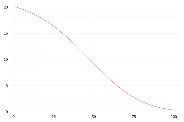
We take the exponent to ensure that the function is positive throughout the time period. What does this look like? We can simple plot the function from 0 to 100 with some random values for the \(\beta _i\)s.

λ(t::Number, params::Array{<:Number}) = exp(params[1] + params[2]*(t/100) + params[3]*(t/100)^2 + params[4]*(t/100)^3)
λ(t::Array{<:Number}, params::Array{<:Number}) = map(x-> λ(x, params), t)

testParams = [3, -0.5, -0.8, -2.9]
maxT = 100

plot(λ(collect(0:maxT), testParams), label=:none)

This looks like something that definitely changes over time. When
\(\lambda(t)\) is high we expect more events and likewise when it is
low there will be fewer events.

Simulating by Thinning

Let us simulate a point process using this intensity function. To do
so we use a procedure called thinning. This can be explained as a
three step process:

  1. Firstly simulate a constant Poisson process with intensity \(\lambda ^\star\) which is greater than \(\lambda (t)\) for all \(t\). This gives the un-thinned events, \(t^*_i\).
  2. For each un-thinned event calculate the probability it will become one of the final events as \(\frac{\lambda (t^*_i)}{\lambda ^\star}\).
  3. Sample from these probabilities to get the final events.

Simple enough to code up in a few lines of Julia.

lambdaMax = maximum(λ(collect(0:0.1:100), testParams)) * 1.1
rawEvents = rand(Poisson(lambdaMax * maxT), 1)[1]
unthinnedEvents = sort(rand(Uniform(0, maxT), rawEvents))
acceptProb = λ(unthinnedEvents, testParams) / lambdaMax
events = unthinnedEvents[rand(length(unthinnedEvents)) .< acceptProb];
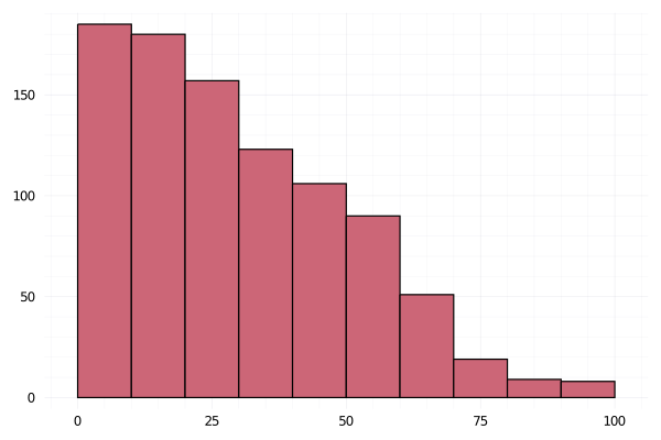
histogram(events,label=:none)

svg

A steady decreasing amount of events following the intensity function from above.

Maximum Likelihood Estimation

The log likelihood of a point process can be written as:

\[\mathcal{L} = \Sigma _{i = 1} ^N \log \lambda (t_i) – \int _0 ^T \lambda (t) \mathrm{d} t\]

Again, easy to write the code for this. The only technical difference is I am using the QuadGK.jl package to numerically integrate the function rather than doing the maths myself. This keeps it simple and also flexible if we decided to change the intensity function later.

function likelihood(params, rate, events, maxT)
    sum(log.(rate(events, params))) - quadgk(t-> rate(t, params), 0, maxT)[1]
end

For maximum likelihood estimation we simply pass this function through to an optimiser and find the maximum point. As optimize actually finds minimum points we have to invert the function.

using Optim
using QuadGK
opt = optimize(x-> -1*likelihood(x, λ, events, maxT), rand(4))
plot(λ(collect(0:maxT), testParams), label="True")
plot!(λ(collect(0:maxT), Optim.minimizer(opt)), label = "MLE")

svg

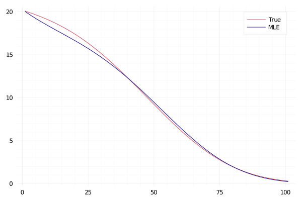
Not a bad result! Our estimated intensity function is pretty close to
the actual function. So now we know that we can both simulate from a inhomogeneous point
process and that our likelihood can infer the correct parameters.

Bayesian Inference

Now for the good stuff. All of the above is needed for the Bayesian inference procedure. If you can’t get the maximum likelihood working for a relatively simple problem like above, adding in the complications of Bayesian inference will just get you knotted up without any results. So with the good results from above let us proceed to the Bayes methods. With the AdvancedHMC.jl package I can use all the fancy MCMC algos and upgrade from the basic Metropolis Hastings sampling.

I’ve shamelessly copied the README from AdvancedHMC.jl and changed the bits needed for this problem.

using AdvancedHMC, ForwardDiff

D = 4; initial_params = rand(D)

n_samples, n_adapts = 5000, 2000

target(x) = likelihood(x, λ, events, maxT) + sum(logpdf.(Normal(0, 5), x))

metric = DiagEuclideanMetric(D)
hamiltonian = Hamiltonian(metric, target, ForwardDiff)

initial_ϵ = find_good_stepsize(hamiltonian, initial_params)
integrator = Leapfrog(initial_ϵ)
proposal = NUTS{MultinomialTS, GeneralisedNoUTurn}(integrator)
adaptor = StanHMCAdaptor(MassMatrixAdaptor(metric), StepSizeAdaptor(0.8, integrator))

samples1, stats1 = sample(hamiltonian, proposal, initial_params, 
                        n_samples, adaptor, n_adapts; progress=true);
samples2, stats2 = sample(hamiltonian, proposal, initial_params, 
                        n_samples, adaptor, n_adapts; progress=true);

Samples done, now to manipulate the results to get the parameter
estimation.

a11 = map(x -> x[1], samples1)
a12 = map(x -> x[1], samples2)
a21 = map(x -> x[2], samples1)
a22 = map(x -> x[2], samples2)
a31 = map(x -> x[3], samples1)
a32 = map(x -> x[3], samples2)
a41 = map(x -> x[4], samples1)
a42 = map(x -> x[4], samples2)

bayesEst = map( x -> mean(x[1000:end]), [a11, a21, a31, a41])
bayesLower = map( x -> quantile(x[1000:end], 0.25), [a11, a21, a31, a41])
bayesUpper = map( x -> quantile(x[1000:end], 0.75), [a11, a21, a31, a41])
density(a21, label="Chain 1")
density!(a22, label="Chain 2")
vline!([testParams[2]], label="True")
plot!(-4:4, pdf.(Normal(0, 5), -4:4), label="Prior")

svg

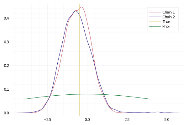
The chains have sampled correctly and are centered around the correct
value. Plus it’s suitably different from the prior, which shows it has
updated with the information from the events.

plot(a11, label="Chain 1")
plot!(a12, label="Chain 2")

svg

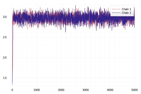
Looking at the convergence of the chains is also positive. So for this
simple model, everything looks like it has worked correctly.

plot(λ(collect(0:maxT), testParams), label="True")
plot!(λ(collect(0:maxT), Optim.minimizer(opt)), label = "MLE")
plot!(λ(collect(0:maxT), bayesEst), label = "Bayes")

svg

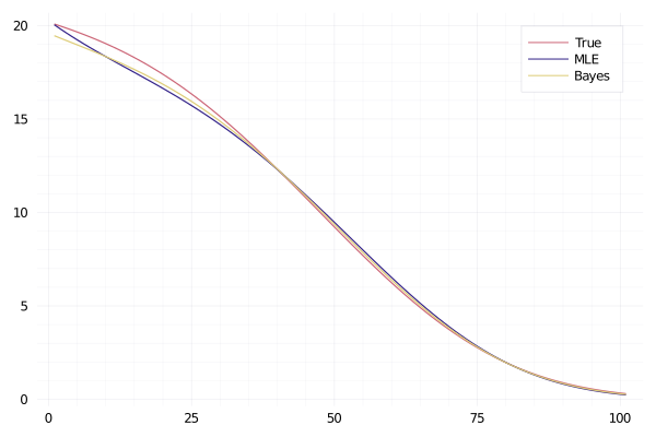
Again, the bayesian estimate of the function isn’t too far from the true intensity. Success!

Conclusion

So what have I learnt after writing all this:

  • AdvancedHMC.jl is easy to use and despite all the scary terms and settings you can get away with the defaults.

What I have hopefully taught you after reading this:

  • Point process simulation through thinning.
  • What the likelihood of a point process looks like.
  • Maximum likelihood using Optim.jl
  • How to use AdvancedHMC.jl for that point process likelihood to get the posterior distribution.