Category Archives: Julia

Sets, chains and rules – part I

By: Julia on μβ

Re-posted from: https://matbesancon.xyz/post/2020-12-23-chains_sets/

Table of Contents

In this post, I will develop the process through which the
MathOptSetDistances.jl
package has been created and evolved. In the second one, I will go over the differentiation part.

MathOptInterface and the motivation

MathOptInterface.jl or MOI
for short is a Julia package to unify structured constrained optimization problems.
The abstract representation of problems MOI addresses is as follows:

$$
\begin{align}
\min_{x}\,\, & F(x) \\\\
\text{s.t.}\,\, & G_k(x) \in \mathcal{S}_k \,\, \forall k \\\\
& x \in \mathcal{X}.
\end{align}
$$

$\mathcal{X}$ is the domain of the decision variables,
$F$ is the objective function, mapping values of the variables to the real line.
The constrained aspect comes from the constraints $G_k(x) \in \mathcal{S}_k$,
some mappings of the variables $G_k$ have to belong to a certain set $\mathcal{S}_k$.
See this recent paper on MOI for more information
on this representation.

The structured aspect comes from the fact that a specific form of $F$, $G$
and $\mathcal{S}$ is known in advance by the modeller. In other words, MOI
does not deal with arbitrary unknown functions or black-box sets.
For such cases, other tools are more adapted.

From a given problem in this representation, two operations can be of interest
within a solution algorithm or from a user perspective:

  1. Given a value for $x$, evaluating a function $F(x)$ or $G(x)$,
  2. Given a value $v$ in the co-domain of $G_k$, asserting whether $v \in S_k$.

The first point is addressed by the function eval_variables in the MOI.Utilities submodule
(documentation).

The second point appears as simple (or at least it did to me) but is trickier.
What tolerance should be set?
Most solvers include a numerical tolerance on constraint violations, should this
be propagated from user choices, and how?

The deceivingly simple feature ended up opening one of the
longest discussions
in the MOI repository.

Fairly straightforward[…]

Optimistic me, beginning of the PR, February 2020

A more meaningful query for solvers is, given a value $v$, what is the
distance from $v$ to the set $\mathcal{S}$:

$$
\begin{align}
(\text{δ(v, s)})\,\,\min_{v_p}\,\, & \text{dist}(v_p, v) \\\\
\text{s.t.}\,\, & v_p \in \mathcal{S}.
\end{align}
$$

The optimal value of the problem above noted $δ(v, s)$ depends on the
notion of the distance taken between two values in the domain $\mathcal{V}$,
noted $dist(\cdot,\cdot)$ here.
In terms of implementation, the signature is roughly:

distance_to_set(v::V, s::S) -> Real

Aside:
this is an example where multiple dispatch brings great value to the design:
the implementation of distance_to_set depends on both the value type V
and the type of set S. See why it’s useful in the
Bonus section.

If $\mathcal{S}$ was a generic set, computing this distance would be as hard as
solving an optimization problem with constraints $v \in \mathcal{S}$ but
since we are dealing with structured optimization, many particular sets have
closed-form solutions for the problem above.

Examples

$\|\cdot\|$ will denote the $l_2-$norm if not specified.

The distance computation problem defined by the following data:

$$
\begin{align}
& v \in \mathcal{V} = \mathbb{R}^n,\\
& \mathcal{S} = \mathbb{Z}^n,\\
& dist(a, b) = \|a – b\|
\end{align}
$$

consists of rounding element-wise to the closest integer.

The following data:

$$
\begin{align}
& v \in \mathcal{V} = \mathbb{R}^n,\\
& \mathcal{S} = \mathbb{R}^n_+,\\
& dist(a, b) = \|a – b\|
\end{align}
$$

find the closest point in the positive orthant, with a result:

$$
v_{p}\left[i\right] = \text{max}(v\left[i\right], 0) \,\, \forall i \in \{1..n\}.
$$

Set projections

The distance from a point to a set tells us how far a given candidate is from
respecting a constraint. But for many algorithms, the quantity of interest is
the projection itself:

$$
\Pi_{\mathcal{S}}(v) \equiv \text{arg} \min_{v_p \in \mathcal{S}} \text{dist}(v, v_p).
$$

Like the optimal distance, the best projection onto a set can often be defined
in closed form i.e. without using generic optimization methods.

We also keep the convention that the projection of a point already in the set is
always itself:
$$
δ(v, \mathcal{S}) = 0 \,\, \Leftrightarrow \,\, v \in \mathcal{S} \,\, \Leftrightarrow \,\, \Pi_{\mathcal{S}}(v) = v.
$$

The interesting thing about projections is that once obtained, a distance
can be computed easily, although only computing the distance can be slightly
more efficient, since we do not need to allocate the projected point.

User-defined distance notions

Imagine a set defined using two functions:
$$
\begin{align}
\mathcal{S} = \{v \in \mathcal{V}\,|\, f(v) \leq 0, g(v)\leq 0 \}.
\end{align}
$$

The distance must be evaluated with respect to two values:
$$
(max(f(v), 0), max(g(v), 0)).
$$

Here, the choice boils down to a norm, but hard-coding it seems harsh and rigid for users.
Even if we plan correctly and add most norms people would expect, someone will
end up with new exotic problems on sets,
complex numbers or function spaces.

The solution that came up after discussions is adding a type to dispatch on,
specifying the notion of distance used:

function distance_to_set(d::D, v::V, s::S)
        where {D <: AbstractDistance, V, S <: MOI.AbstractSet}
    # ...
end

which can for instance encode a p-norm or anything else.
In many cases, there is no ambiguity, and the package defines DefaultDistance()
exactly for this.

Bonus

If you are coming from a class-based object-oriented background, a common
design choice is to define a Set abstract class with a method project_on_set(v::V) to implement.
This would work for most situations, since a set often implies a domain V.
What about the following:

# Projecting onto the reals (no-op)
project_on_set(v::AbstractVector{T}, s::Reals) where {T <: Real}

# Projecting onto the reals (actual work)
project_on_set(v::AbstractVector{T}, s::Reals) where {T <: Complex}

Which “class” should own the implementation in that case?
From what I observed, libraries end up with either an enumeration:

if typeof(v) == AbstractVector{<:Reals}
    # ...
elseif # ...
end

or when the number of possible domains is expected to be low, with several methods:

# in the set class Reals
function project_real(v::AbstractVector{T}) where {T <: Real}
end

function project_complex(v::AbstractVector{T}) where {T <: Complex}
end

function project_scalar(v::T) where {T <: Real}
end

As a last remark, one may wonder why would one define trivial sets as the MOI.Reals
or the MOI.Zeros. A good example where this is needed is the polyhedral cone:
$$
A x = 0
$$
with $x$ a vector. This makes more sense to define $Ax$ as the function and
MOI.Zeros as the set.

Creating and Deploying your Julia Package Documentation

By: DSB

Re-posted from: https://medium.com/coffee-in-a-klein-bottle/creating-and-deploying-your-julia-package-documentation-1d09ddc90474?source=rss-8bd6ec95ab58------2

A tutorial on how to create and deploy your Julia Package documentation using Documenter.jl and GitHub Actions.

If you are developing a new package for Julia, you might’ve followed the steps in this article, and is now wondering how to create the documentation for your package. Well, this is what this article is for. Here, our new package is also called VegaGraphs.jl, which is a package that I’m developing at the moment.

In this tutorial I’ll be using the package Documenter.jl together with the GitHub Actions plugin. The Documenter.jl package will help us create the documentation, and the GitHub Actions plugin will create a bot for us that will publish our documentation on our GitHub page.

1. Creating Docstring

First of all, when you write the functions in your package, above each function you should write a Docstring explaining the arguments used in the function, what the function does, etc.

# Example of function inside ./src/VegaGraphs.jl
"""
MyFunction(x,y)
This is an example of Docstring. This function receives two 
numbers x and y and returns the sum of the squares.
```math
x^2 + y^2
```
"""
function MyFunction(x,y)
return x^2+y^2
end

Note that you should use triple quotes, and place the text right above the function you are documenting. Also, you may use LaTeX to write math equations, as shown in the lines:

```math
x^2 + y^2
```

When you generate your documentation, this equation will be properly rendered, and you will have a beautiful mathematical equation.

2. Setting up Documenter.jl

Next we must set up the Documenter.jl. To do this, first create a folder named docs and inside of it create a file named make.jland another folder named ./src . Your package folder should look something like this:

VegaGraphs/
├── docs/
│ └── make.jl
│ └── src/
├── src/
│ └── VegaGraphs.jl
...

Inside the make.jl file we will write the code that Documenter.jl will use to create a nice webpage for our documentation. Inside make.jl write the following (changing the name of the package from VegaGraph to yours):

# Inside make.jl
push!(LOAD_PATH,"../src/")
using VegaGraphs
using Documenter
makedocs(
sitename = "VegaGraphs.jl",
modules = [VegaGraphs],
pages=[
"Home" => "index.md"
])
deploydocs(;
repo="github.com/USERNAME/VegaGraphs.jl",
)

Most of the code here is self-explanatory. You are defining the name the website for the documentation, the module which you will be documenting, and the pages your website will have. For now, our documentation will only have “Home”, and the information that will be on this page will be inside the index.m file.

Inside the ./docs/src you need to create the file named index.md. This is a markdown file where you will write how the “Home” page should look like. Here is an example:

# VegaGraphs.jl
*The best summation package.*
## Package Features
- Sum the squares of two numbers
## Function Documentation
```@docs
MyFunction
```

Everything here should be familiar to you if you know markdown. The only thing that looks different are the last 4 lines. Here is where our Docstring comes in. The Documenter.jl package will take the Docstring from the function MyFunction and place where we wrote:

```@docs
MyFunction
```

As your create new functions, just add more of this to your index.md , and you will rapidly create your package’s documentation.

The final step in regards to Documenter.jl is to build the whole thing:

# from your terminal,inside the ./docs/src
# Remember to install Documenter.jl before running this
julia make.jl

After running this command, a new folder called build will be created inside the docs , and this folder will contain all the html files for your documentation. You may now open this folder

3. Deploying your Documentation with GitHub Actions

Your website containing the documentation for the package is already created, and you may host the webpages using any method you want. In this section, I’ll then explain how to use GitHub Actions to automatically publish the documentation using GitHub pages.

Assuming you followed this article here on how to develop your package, you already have GitHub Actions working on the background. What you must do now is create a file named Documentation.yml inside the .github/workflows folder. Inside this file, you should have something like this:

name: Documentation
on:
push:
branches:
- master
tags: '*'
pull_request:
jobs:
build:
runs-on: ubuntu-latest
steps:
- uses: actions/checkout@v2
- uses: julia-actions/setup-julia@latest
with:
version: '1.5'
- name: Install dependencies
run: julia --project=docs/ -e 'using Pkg; Pkg.develop(PackageSpec(path=pwd())); Pkg.instantiate()'
- name: Build and deploy
env:
GITHUB_TOKEN: ${{ secrets.GITHUB_TOKEN }} # For authentication with GitHub Actions token
run: julia --project=docs/ docs/make.jl

You can pretty much copy and past the code above, and the next time you push new commits to your repository, the bot will run and generate the documentation. Also, note that it will create a branch named “gh-pages”. This is the branch containing the webpages for the documentation.

To use GitHub pages for hosting our documentation, we must enable GitHub pages on the repository containing the package. To do this, just go to the repository GitHub’s page, click on setttings , scroll down to the “GitHub Pages” section and enable it.

Example showing how to enable the hosting of your documentation

After doing all this, your documentation will be available at “https://username.github.io/VegaGraphs.jl/dev.

And you now has a beautiful website for your documentation.

Example of documentation page generated with Documenter.jl


Creating and Deploying your Julia Package Documentation was originally published in Coffee in a Klein Bottle on Medium, where people are continuing the conversation by highlighting and responding to this story.

Converting an Edward Tutorial (Python) to Flux (Julia)

By: Dean Markwick's Blog -- Julia

Re-posted from: https://dm13450.github.io/2020/12/19/EdwardAndFlux.html

Here I’ll be showing you how to take a model built in Python with
Edward, convert it into Julia and perform the same type of inference
using Flux and Turing.jl.


Enjoy these types of posts? Then sign up for my newsletter.


Edward is a probabilistic programming language like Stan, PyMC3
and Turing.jl. You write a model and can perform statistical
inference on some data. Edward is a more ‘machine learning’ focused than Stan as
you can build neural nets and all the fun, modern techniques that the cool kids
are using. Flux.jl takes a similar ‘machine learning’ approach but this
time in Julia. Flux can build neural nets and also much
more. There is an intersection here between Edward and Flux, so it
makes sense to think that you can perform similar tasks. That is the whole point of this blog post, translating this
Edward tutorial: http://edwardlib.org/getting-started into Julia code
for Flux. So anyone reading this can get an idea of:

  • what Flux is all about,
  • how the Python Edward code can be transformed into Julia,
  • how to build a simple neural nets and infer the parameters in a Bayesian way.

I’ll start off by reproducing the model in Flux before calling on
Turing to do the Bayes bit. This is my first time writing about Flux,
so hopefully you’ll find this useful if it is also your first foray into doing some machine learning in Julia.

using Flux
using Plots
using Distributions

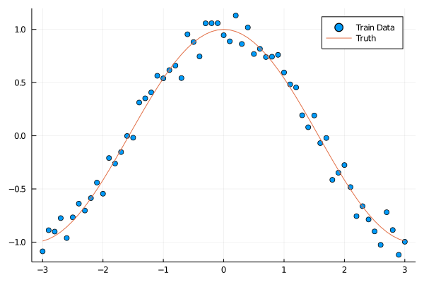
The original tutorial wants to learn the cos function of which we add some Gaussian noise.

f(x) = cos(x) + rand(Normal(0, 0.1))

xTrain = collect(-3:0.1:3)
yTrain = f.(xTrain)
plot(xTrain, yTrain, seriestype=:scatter, label="Train Data")
plot!(xTrain, cos.(xTrain), label="Truth")

True data from the cos function

To build the neural net we chain two dense layers with tanh nonlinearities inbetween the layers. We use the mean square error as our loss function which we minimise using gradient descent. This is the most basic way in which you can build and train the neural net. Directly replicating what Edward does comes later, for now we just want to get things working.

With Flux you can specify what type of loss quite easily, with a list
of all that comes prepackaged found here
https://fluxml.ai/Flux.jl/stable/models/losses. But if none of those
take your fancy you can write your own and pass a simple Julia
function.

model = Chain(Dense(1, 2, tanh), Dense(2, 1))
loss(x, y) = Flux.Losses.mse(model(x), y)
optimiser = Descent(0.1);

Likewise for the optimiser. I’ve chose gradient descent, but again,
you can switch it out for a more advanced approach, such as ADAM. See
if any of those listed here
https://fluxml.ai/Flux.jl/stable/training/optimisers/ take your
fancy.

In short, the neural net takes one value as an input, passes through to two nodes on the hidden layer with a tanh activation function before outputting a single value as the output.

We now set up the training data. We take 100 random normal samples as our inputs, use our f function to generate the outputs and then repeat the dataset 100 times.

x = rand(Normal(), 100)
y = f.(x)
train_data = Iterators.repeated((Array(x'), Array(y')), 100);

We train the model for 10 epochs.

Flux.@epochs 10 Flux.train!(loss, Flux.params(model), train_data, optimiser)

Which takes no time at all to complete. We now want to make sure the
results are sensible and it has actually learnt the underlying
function.

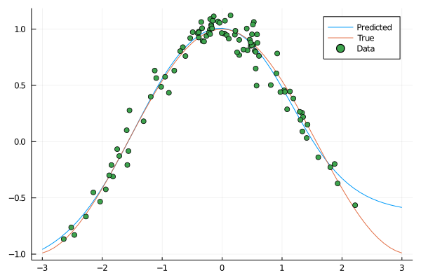
yOut = zeros(length(xTrain))
for (i, x) in enumerate(xTrain)
    yOut[i] = model([xTrain[i]])[1]
end

plot(xTrain, yOut, label="Predicted")
plot!(xTrain, cos.(xTrain), label="True")
plot!(x, y, seriestype=:scatter, label="Data")

Predicted cruve from Flux

Everything looking good. Our neural net has found something similar to the true function, so hopefully you are convinced that we can now add a layer of complexity. Slight disagreement around the tails, but that is where we are lacking some data, so not too big of a deal.

Bayesian Neural Networks with Flux and Turing

All the above captured the spirit, but not the whole point of the
Edward tutorial, which is to create a Bayesian neural net. With a
Bayesian neural net there is a probability distribution over the
weights, rather than just singular values to maximise. In Julia, we
have to call upon our old friend Turing.jl. The Turing team have
written about Bayesian neural networks. I’ve taken some of that code and shuffled it about for this application.

using Turing

Firstly, have the parameters for each of the layers of the neural net. In total there are 6 parameters for the two layer model, so using the unpack function we take a vector of length 6 and break it up into the weights and biases for each layer which we then build in the nn_forward function.

function unpack(nn_params::AbstractVector)
    W₁ = reshape(nn_params[1:2], 2, 1);   
    b₁ = reshape(nn_params[3:4], 2)
    
    W₂ = reshape(nn_params[4:5], 1, 2); 
    b₂ = [nn_params[6]]
    
    return W₁, b₁, W₂, b₂
end

function nn_forward(xs, nn_params::AbstractVector)
    W₁, b₁, W₂, b₂ = unpack(nn_params)
    nn = Chain(Dense(W₁, b₁, tanh), Dense(W₂, b₂))
    return nn(xs)
end

These utility functions mean that we are tearing down the neural net and rebuilding it with the new parameters with each iteration. Turing deals with finding the best parameters by doing the Bayesian sampling (see my previous post on Hamilton MCMC sampling).

We think the 6 parameters of the neural net are drawn from a multivariate normal distribution and the parameters are all uncorrelated with each other. The observations are also from a normal distribution with mean from the neural net and variance \(\sigma\).

alpha = 0.1
sig = sqrt(1.0 / alpha)

@model bayes_nn(xs, ys) = begin
    
    nn_params ~ MvNormal(zeros(6), sig .* ones(6)) #Prior
    
    preds = nn_forward(xs, nn_params) #Build the net
    sigma ~ Gamma(0.01, 1/0.01) # Prior for the variance
    for i = 1:length(ys)
        ys[i] ~ Normal(preds[i], sigma)
    end
end;

Model built, we now want to use the NUTS algorithm to sample from the
posterior. Again, like Flux, you can use other sampling methods such as HMC
or Metropolis-Hastings.

N = 5000
ch1 = sample(bayes_nn(hcat(x...), y), NUTS(0.65), N);
ch2 = sample(bayes_nn(hcat(x...), y), NUTS(0.65), N);

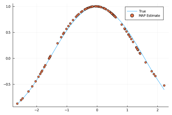
We sample from posterior 5,000 times with two chains to check the convergence later. When selecting the final parameters we chose those that maximise the log posterior of the model. For each of the datapoints we add the prediction from the neural net.

lp, maxInd = findmax(ch1[:lp])

params, _ = ch1.name_map
bestParams = map(x-> ch1[x].data[maxInd], params[1:6])
plot(x, cos.(x), seriestype=:line, label="True")
plot!(x, Array(nn_forward(hcat(x...), bestParams)'), 
      seriestype=:scatter, label="MAP Estimate")

MAP estimate of the function

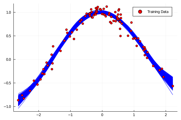
We can also sample from this posterior distribution by looking at the different parameters from the sampling process.

xPlot = sort(x)

sp = plot()

for i in max(1, (maxInd[1]-100)):min(N, (maxInd[1]+100))
    paramSample = map(x-> ch1[x].data[i], params)
    plot!(sp, xPlot, Array(nn_forward(hcat(xPlot...), paramSample)'), 
        label=:none, colour="blue")
    
end

plot!(sp, x, y, seriestype=:scatter, label="Training Data", colour="red")

sp

Posterior draws of the function

Again, looking sensible and representing the true underlying
function. Plus as we have done this using Bayes, we have a good
visualisation of the uncertainty of the model too.

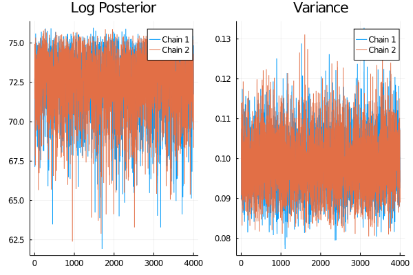
And then finally we can assess how the chains of the model look and make a judgement on whether they have converged.

lPlot = plot(ch1[:lp], label="Chain 1", title="Log Posterior")
plot!(lPlot, ch2[:lp], label="Chain 2")

sigPlot = plot(ch1[:sigma], label= "Chain 1", title="Variance")
plot!(sigPlot, ch2[:sigma], label="Chain 2")

plot(lPlot, sigPlot)

Chain convergence

Both chains are looking like they have converged, so we can trust our sampling process.

Conclusion

I actually surprised myself with how easy it was to build and sample
from the neural net in a Bayesian manner. I originally thought that I
would only be able to replicate the model using frequentist methods,
but not the Bayes steps. This just goes to show what a great job the Turing.jl team have done, making the whole model building and sampling simple.
So after reading this you can extended these models to bigger
and badder neural nets if that is what your problem needs. Easily swapping out
losses, optimisers and posterior sampling methods as needed.

This post also shows how easy it is to translate back and forth
between the different machine learning libraries and even programming
languages, although there is not too much of a difference between
Julia and Python. So if anyone out there is reading this trying to
decide on what language to pick up, I’d be biased and say Julia, but
really, you’ll be fine with either one.