Category Archives: Julia

First Steps #4: Digging Into DataFrames

By: Josh Day

Re-posted from: https://www.juliafordatascience.com/first-steps-4-dataframes/

First Steps #4: Digging Into DataFrames

DataFrames.jl provides the most widely used tabular data structure in Julia.  In this post we'll explore DataFrames using sample data from RDatasets.jl (and we'll plot stuff using StatsPlots).

A rather timely event: DataFrames.jl has reached version 1.0!

⚙️ Setup

First, install DataFrames and RDatasets via Pkg Mode (]) in the REPL:

(@v1.6) pkg> add DataFrames RDatasets

Now load both packages along with the diamonds dataset from R's ggplot2 package.  The diamonds data contains price/size/quality information on 53,940 different diamonds.  

julia> using DataFrames, RDatasets

julia> df = dataset("ggplot2", "diamonds")
53940×10 DataFrame
   Row │ Carat    Cut        Color  Clarity  Depth    Tabl ⋯
       │ Float64  Cat…       Cat…   Cat…     Float64  Floa ⋯
───────┼────────────────────────────────────────────────────
     1 │    0.23  Ideal      E      SI2         61.5     5 ⋯
     2 │    0.21  Premium    E      SI1         59.8     6
     3 │    0.23  Good       E      VS1         56.9     6
     4 │    0.29  Premium    I      VS2         62.4     5
     5 │    0.31  Good       J      SI2         63.3     5 ⋯
     6 │    0.24  Very Good  J      VVS2        62.8     5
     7 │    0.24  Very Good  I      VVS1        62.3     5
     8 │    0.26  Very Good  H      SI1         61.9     5
   ⋮   │    ⋮         ⋮        ⋮       ⋮        ⋮        ⋮ ⋱

🚀 DataFrames Quickstart

  • Variables (columns) of a Dataframe can be referenced either by strings or symbols, e.g. "I am a string" and :I_am_a_symbol.

Make a Copy of a Column

df[:, "Carat"]

df[:, :Carat]

Extract a Column

  • These commands retrieve the exact data held in the DataFrame.  Warning!  Making a change to the extracted data will change the values in DataFrame.
df.Carat

df[!, "Carat"]

Selecting a Subset of Columns

select(df, "Carat")

select(df, ["Carat", "Cut"])

Filtering a Subset of Rows

The syntax x -> do something with x is an anonymous function (sometimes called lambda expression).  The filter function will apply a function to each row and return back a DataFrame for the rows that returned true.

filter(row -> row.Carat > 1, df)
  • We can also use indexing (with broadcasting) rather than filter:
df[df.Carat .> 1, :]
  • For functions that accept a function as its first argument, Julia's do-block syntax can help you clean up your code.  Here we are using &&, the logical "and" operator, to create multiple filter conditions.
filter(x -> x.Carat > 1 && x.Cut == "Premium" && x.Color == "J" && 5000 <= x.Price <= 6000, df)

# Same as above, but with do-block
filter(df) do x 
    x.Carat > 1 && 
        x.Cut == "Premium" && 
        x.Color == "J" &&
        5000 <= x.Price <= 6000
end

You can now do several essential DataFrame tasks:

  • Get a single column
  • Choose a subset of columns
  • Choose a subset of rows

Next we'll use groupby and combine to apply functions across groups of data.

🤔 How does Price relate to Cut?

We are big on learning by example, so let's start by answering this relatively simple question.  First things first: What do the Price and Cut variables look like?

julia> df.Price
53940-element Vector{Int32}:
  326
  326
    ⋮
 2757
 2757

julia> df.Cut
53940-element CategoricalArrays.CategoricalArray{String,1,UInt8}:
 "Ideal"
 "Premium"
 ⋮
 "Premium"
 "Ideal"
  • Price: The cost in US Dollars.
  • Cut: The rating of cut quality.  In order (best-to-worst): "Ideal", "Premium" "Very Good", "Good", and "Fair".  Side note: The data is stored in a CategoricalArray, which uses less memory than storing each element as a separate String.

Using groupby

We can use the groupby function to group our data by the "Cut" variable.

gdf = groupby(df, :Cut)

Using our grouped DataFrame, we can then apply a function to a variable in each group using combine.  Let's get the average Price for each level of Cut:

julia> using Statistics # for `mean`

julia> combine(gdf, :Price => mean)
5×2 DataFrame
 Row │ Cut        Price_mean
     │ Cat…       Float64
─────┼───────────────────────
   1 │ Fair          4358.76
   2 │ Good          3928.86
   3 │ Very Good     3981.76
   4 │ Premium       4584.26
   5 │ Ideal         3457.54

Now we know what the distribution center is for each Cut, but what about the spread and shape?

📊 Using StatsPlots

The StatsPlots package adds functionality and plot recipes to Plots.jl.  We'll use it to do the grouping for us so that we don't need groupby.  First, add StatsPlots:

(@v1.6) pkg> add StatsPlots

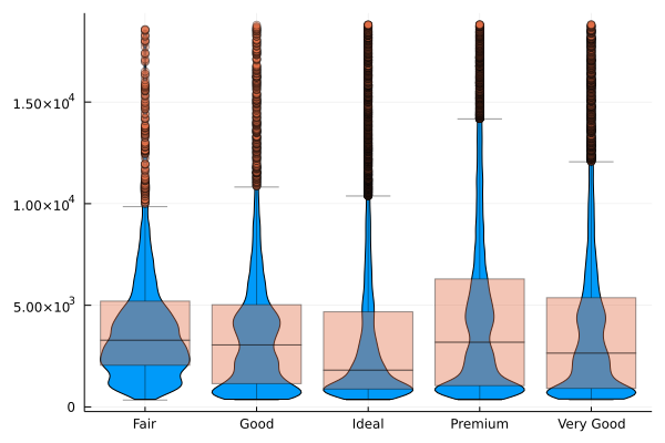
Next, use the @df <dataframe> <plot command> syntax to create a violin plot overlaid with a box plot for each level of Cut.

julia> @df df violin(string.(:Cut), :Price, lab="")

julia> @df df boxplot!(string.(:Cut), :Price, alpha=.4, lab="")
First Steps #4: Digging Into DataFrames
Price vs. Cut

Things to note in the code/plot above:

  • The @df macro will replace Symbols with the associated DataFrame columns.
  • We must use string.(:Cut) because Plots/StatsPlots doesn't know how to work with CategoricalArrays directly.
  • We use boxplot! (instead of boxplot) to add a new series to the existing plot.
  • We set lab (shorthand for label) to "" to avoid adding an entry to the plot legend.  If all legend entries are blank, the legend will not appear.
  • We use alpha=.4 to set the opacity of the boxplot so that it doesn't cover up the violin in the layer beneath it.

From our plot, we can see the distributions are all similarly skewed with a long right tail.  Some Cuts (Good, Premium, and Very Good) are bimodal (they have two "peaks").  However, we are ignoring some important factors (such as how Carat and Color affect the price!), so we shouldn't make any conclusions based solely on this plot.

🚀 That's It!

You now know how to do a little bit of data wrangling with DataFrames.  What do you want to learn about next?

Enjoying Julia For Data Science?  Please share us with a friend and follow us on Twitter at @JuliaForDataSci.
Additional Resources

Talk ‘Introduction to Julia and Trixi, a numerical simulation framework for hyperbolic PDEs’ on 2021-04-27

By: Hendrik Ranocha -- Julia blog

Re-posted from: https://ranocha.de/blog/Intro_Julia_Trixi/

I gave a talk
Introduction to Julia and Trixi, a numerical simulation framework for hyperbolic PDEs
in the Applied Mathematics Seminar, University of Münster, on Tuesday, 2021-04-27, 10:00 CEST.
The announcement including details how to participate is available online.

Abstract

Julia is a modern high-level programming language developed specifically
with scientific computing in mind. Trixi is a
numerical simulation framework for hyperbolic conservation laws written in Julia. A key objective
for the framework is to be useful to both scientists and students. Therefore, next to having an
extensible design with a fast implementation, Trixi is focused on being easy to use for new or
inexperienced users, including the installation and postprocessing procedures.

This presentation is a live demonstration of Julia and Trixi. Firstly, we introduce Julia and
demonstrate some of its design principles. This introduction is aimed at researchers in
numerical analysis with previous programming experience. Next, we show how to use Trixi
for setting up and running simulations, how to visualize the results, and how to extend Trixi
with new functionality. We demonstrate how key design principles of Julia are used in Trixi
and the Julia package ecosystem, e.g. to enable automatic differentiation through a complete
simulation involving hyperbolic conservation laws.

The presentation is
available as a Jupyter notebook,
including information how to set up everything.

Accidentally Quadratic with DataFrames in Julia

By: Dean Markwick's Blog -- Julia

Re-posted from: https://dm13450.github.io/2021/04/21/Accidentally-Quadratic.html

using DataFrames, DataFramesMeta
using BenchmarkTools
using Plots

A post recently done the rounds where it looks like GTA had a bad
implementation of an algorithm that scaled in a quadratic fashion (How I cut GTA Online loading times by 70%),
which echoed a Bruce Dawson quote article about how it is common for
quadratically efficient processes to end up in production.
Quadratic
algorithms are fast enough when testing but once in production all of
a sudden the performance issues catch up with you and your sat with a
very inefficient process.

Well that happened to me.

Every month I recalibrate a model using the latest data pulled from a
database. I take this raw data and generate some features, fit a model
and save down the results. One of those operations is to match all the
id’s with the old data and new data to work out which trades need new features needed to be generated.

Basically, imagine I have a dataframe, and I want to find all the rows
that match some values. In this mock example, column B contains the
IDs and I’ve some new IDs that I want to filter the dataframe for.

I’ll create a large mock dataframe as an example.

N = 1000000
df = DataFrame(A = rand(N), B = 1:N);

My slow implementation use the DataFramesMeta package and used the broadcasted in function to check whether each value was in the new ids. This worked without a hitch last month, but then all of a sudden seemed to be incredibly slow. This was strange as I hadn’t changed anything, did the usual reboot of the machine and start afresh but it was still painfully slow.

function slow(df, ids)
  @where(df, in(ids).(:B))
end

After a quick profiling, I found that it was the above function that
was the bottleneck. So I refactored it to remove the DataFramesMeta dependancy and just used the base functions.

function quick(df, ids)
  df[findall(in(ids), df.B), :]
end

Thankfully this solved the issue, was much quicker and allowed my
process to complete without a hitch. This got me thinking, how slow was my originally implementation and how much different is the new version. So onto the benchmarking.

Using the BenchmarkTools.jl package I can run multiple iterations of each function across larger and larger IDs samples.

nSamps = [1, 10, 100, 1000, 10000, 100000, 1000000]
resQuick = zeros(length(nSamps))
resSlow = zeros(length(nSamps))

for (i, n) in enumerate(nSamps)
  ids = collect(1:n) 
    
  qb = @benchmark quick($df, $ids)
  sb = @benchmark slow($df, $ids)
    
  resQuick[i] = median(qb).time
  resSlow[i] = median(sb).time
end

I’ve made sure that I compiled the original function before starting
this benchmarking too.

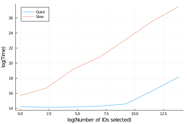
plot(log.(nSamps), log.(resQuick), label="Quick", legend=:topleft, xlabel="log(Number of IDs selected)", ylab="log(Time)")
plot!(log.(nSamps), log.(resSlow), label="Slow")

svg

The difference in performance in remarkable. The quick function
is pretty much flat and just a slight increase towards the large sizes
in this log-log plot, whereas the slow version is always increasing. When we model the slow implementation performance as a power law we find that it is not quite quadratic, but more importantly, we can see that the faster method is pretty much constant, so a much scalable solution.

using GLM
lm(@formula(LogTime ~ LogSamps),
     DataFrame(LogSamps = log.(nSamps), LogTime=log.(resSlow)))
StatsModels.TableRegressionModel{LinearModel{GLM.LmResp{Vector{Float64}}, GLM.DensePredChol{Float64, LinearAlgebra.CholeskyPivoted{Float64, Matrix{Float64}}}}, Matrix{Float64}}

LogTime ~ 1 + LogSamps

Coefficients:
─────────────────────────────────────────────────────────────────────────
                 Coef.  Std. Error      t  Pr(>|t|)  Lower 95%  Upper 95%
─────────────────────────────────────────────────────────────────────────
(Intercept)  15.1134     0.275726   54.81    <1e-07  14.4046    15.8221
LogSamps      0.885168   0.0332117  26.65    <1e-05   0.799794   0.970541
─────────────────────────────────────────────────────────────────────────

When I first come across this issue I was ready to book out my week to rewriting the data functions to iron out any of the slow downs, so I was pretty happy that rewriting that one function made everything manageable.