Category Archives: Julia

Gaussian processes and linear regression

By: Oisin Fitzgerald

Re-posted from: https://oizin.github.io/posts/gp-linear/index.html

Gaussian processes and linear regression

Oisín Fitzgerald, May 2021

A look at section 6.4 of:

Bishop C.M. (2006). Pattern recognition and machine learning. Springer.

https://www.microsoft.com/en-us/research/publication/pattern-recognition-machine-learning/

Basically this post goes through (Bayesian) linear regression from a Gaussian process space point of view with some example Julia code to make things concrete.

Update (10/11/2021): Deleted "estimating the hyperparameters" section for now as it was too short and had no examples.

Overview

The dominant approach to solving regression problems in machine learning today is finding the parameters \(w\) of a model \(M_w\) that minimise a loss function \(L\) by optimally combining a set of basis vectors. These basis vectors can be the original data \(x_n\) or some transformation \(z_n = \phi(x_n)\) where \((y_n,x_n)\) is the \(n^{th}\) output-input pair \(n \in \{1,…,N\}\) and \(x_n\) is length \(p\) (the number of features). For example:

  • Linear regression: find the best set of weights \(w\) that minimise mean square error \(\left\Vert Y – X w \right\Vert\) giving us predictions \(y_n = w^t x_n\).

  • Deep learning: at the other extreme of complexity we can think of deep learning as learning both the basis vectors and the weights. In a network with \(L\) layers the outputs and weights of the final layer are \(z_L\) and \(w_L\) giving us \(y_n = w_L^t z_L(x_n)\).

With Gaussian processes with are going to switch from thinking in terms of locating which parameters are most likely to have generated the data to considering the data a finite sample from a function that has particular properties. The parameters and function space viewpoint are not conflicting, for example for linear regression:

  1. Parameter space view: \(y\) is a combination of basis functions with the weights being from a mltivariate normal distribution.

  2. Function space view: \(y(x_n)\) is a sample from a family of functions where any finite sample of points \(\{y_1,…,y_N\}\) follow a multivariate normal distibution.

From the parameter to function space view

To fully see the connection let's go from the parameter space view to the function space view for linear regression. The model is

\[y(x_n) = w^t x_n\]

In matrix form the above is written as \(Y = X w\), with each row of the \(N \times p\) matrix \(X\) made up of the \(N\) individual observations \(x^t_n\), each a vector of length \(p+1\), the number of features plus one (to have an intercept term). The prior distribution on our weights \(w\) reflects a lack of knowledge about the process

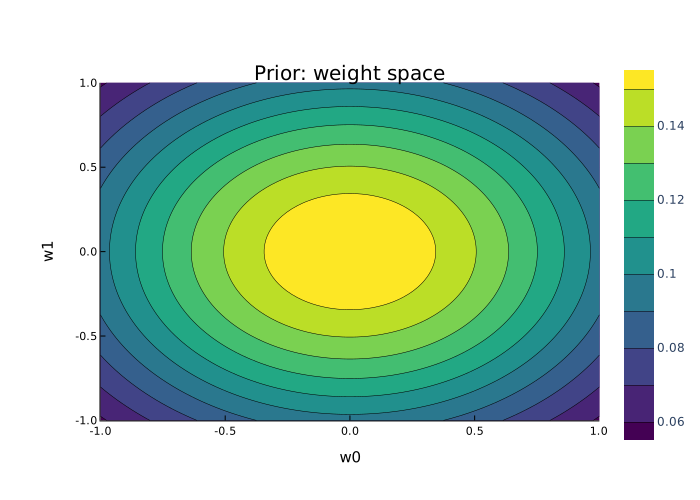
\[w \sim N(0,\alpha^{-1}I)\]

For example if there is one input we have \(w = (w_0, w_1)^t\) and setting \(\alpha = 1.0\) (arbitrarily) the prior looks like the graph below.

using Plots, Random, Distributions, LinearAlgebra
plotlyjs()
Random.seed!(1)
α = 1.0
d = MvNormal([0,0], (1/α)*I)
W0 = range(-1, 1, length=100)
W1 = range(-1, 1, length=100)
p_w = [pdf(d, [w0,w1]) for w0 in W0, w1 in W1]
contourf(W0, W1, p_w, color=:viridis,xlab="w0",ylab="w1",title="Prior: weight space")
Since we treat input features (the x's) as constants this implies a prior distribution for the output

\[y \sim N(0,\alpha X^t X)\]

From the function space view we can randomly sample functions at finite spacings \(\mathfrak{X} = \{x_1,…,x_N\}\) from the prior.

Random.seed!(1)
x1 = range(-1, 1, length=100)
X = [repeat([1],100) x1]
d = MvNormal(repeat([0],100), (1/α)*X*transpose(X) + 1e-10*I)
p = plot(x1,rand(d),legend=false,seriestype=:line,title="Prior: function space",xlabel="x",ylabel="y")
for i in 1:20
    plot!(p,x1,rand(d),legend=false,seriestype=:line)
end
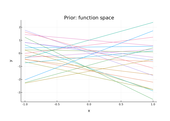
The matrix \(K = \text{cov}(y) = \alpha^{-1} X^t X\) is made up of elements \(K_{nm} = k(x_n,x_m) = \frac{1}{\alpha}x_n^t x_m\) with \(k(x,x’)\) the kernel function. Notice that the kernel function \(k(x,x’)\) returns the variance for \(x = x’\) and covariance between \(x\) and \(x’\) otherwise. Also that we are talking here about the covariance between observations, not features. \(K\) is a \(N \times N\) matrix and so can be quite large. There are many potential kernel functions other than \(k = x^tx\) but that's for another day.

Modelling data with straight lines

We have a prior on \(y\) and then we observe some data. Let assume there is noise in the data so we observe

\[t_n = y(x_n) + \epsilon_n\]

with \(\epsilon_n \sim N(0,\beta)\) random noise that is independent between observations and \(t = \{t_1,…,t_N\}\) the observed output values for input features \(x_n\).

Random.seed!(1)
n = 10
x1 = range(-1, 1, length=n)
X = [repeat([1],n) x1]
β = 0.01
d = MvNormal(repeat([0],n), (1/α)*X*transpose(X) + β*I)
y = rand(d) 
p = scatter(x1,y,legend=false,title="Observed data",xlabel="x",ylabel="y")
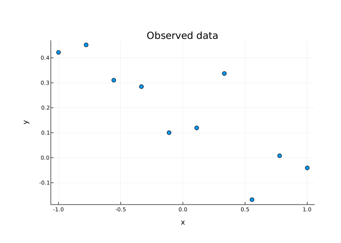
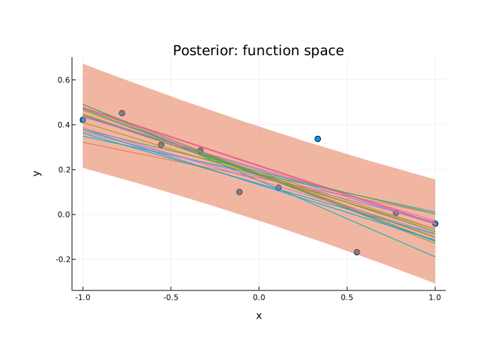
At this point in practise we could estimate the noise parameter \(\beta\), but lets come back to that. For now assume we know that \(\beta = 0.01\). It is worth remember there are no weights giving us the intercept, slope etc but we can sample from our distribution of \(y|t\) or \(t*|t\) or given the observed data. Because our interest is in predicting for new observations we'd like to estimate the posterior \(p(t*|t,x,x*)\) for any future input \(x*\). It turns out the posterior for for any \(t*\) is another normal distribution which is coded below.

p = scatter(x1,y,legend=false,
            title="Posterior: function space",xlabel="x",ylabel="y")# new X's over which to predict
xs = range(-1, 1, length=100)
Xs = [repeat([1],100) xs]
ys = zeros(100)# get ready to construct posterior
σ2 = zeros(100)
C = (1/α)*X*transpose(X) + β*I
Cinv = inv(C)# one prediction at a time 
for i in 1:100
    k = X * Xs[i,:]
    c = Xs[i,:]' * Xs[i,:] + β
    ys[i] = (k' * Cinv) * y
    σ2[i] = c - (k' * Cinv) * k
end
plot!(p,xs,ys, ribbon=(2*sqrt.(σ2),2*sqrt.(σ2)), lab="estimate")
plot!(p,xs,ys)# noise free samples from the posterior
# all predictions at once
m = (Xs * X') * Cinv * y
CV = (Xs * Xs') - (Xs * X') * Cinv * (X * Xs')
CV = Symmetric(CV) + 1e-10*I
d = MvNormal(m, Symmetric(CV) + 1e-10*I)
for i in 1:20
    plot!(p,xs,rand(d),legend=false,seriestype=:line)
end
The order of join and grouping result in DataFrames.jl

By: Blog by Bogumił Kamiński

Re-posted from: https://bkamins.github.io/julialang/2021/04/30/roworder.html

Introduction

Today I want to focus on an issue that is often not noticed by users when
working DataFrames.jl, but in some cases it it might be relevant.

The subject is the order of join and grouping operations result in
DataFrames.jl. The key point of the post is that this order depends on several
factors, so it is simplest to assume that it is undefined.
I am not going to list all cases in my examples, but just focus on showing
the fact as in the future the order might change.

In this post I am using Julia 1.6.1 and DataFrames.jl 1.0.1.

Joins

Consider the following example of innerjoin:

julia> using DataFrames

julia> df1 = DataFrame(x=[2, 3, 1, 4], id1=1:4)
4×2 DataFrame
 Row │ x      id1
     │ Int64  Int64
─────┼──────────────
   1 │     2      1
   2 │     3      2
   3 │     1      3
   4 │     4      4

julia> df2 = DataFrame(x=[1, 3, 2, 5, 6], id2=1:5)
5×2 DataFrame
 Row │ x      id2
     │ Int64  Int64
─────┼──────────────
   1 │     1      1
   2 │     3      2
   3 │     2      3
   4 │     5      4
   5 │     6      5

julia> innerjoin(df1, df2, on=:x)
3×3 DataFrame
 Row │ x      id1    id2
     │ Int64  Int64  Int64
─────┼─────────────────────
   1 │     1      3      1
   2 │     3      2      2
   3 │     2      1      3

julia> innerjoin(df2, df1, on=:x)
3×3 DataFrame
 Row │ x      id2    id1
     │ Int64  Int64  Int64
─────┼─────────────────────
   1 │     1      1      3
   2 │     3      2      2
   3 │     2      3      1

As you can see currently the row order in the result of innerjoin is taken
from the longer table.

Now consider outerjoin (similar results are for leftjoin and rightjoin):

julia> outerjoin(df1, df2, on=:x)
6×3 DataFrame
 Row │ x      id1      id2
     │ Int64  Int64?   Int64?
─────┼─────────────────────────
   1 │     1        3        1
   2 │     3        2        2
   3 │     2        1        3
   4 │     4        4  missing
   5 │     5  missing        4
   6 │     6  missing        5

julia> outerjoin(df2, df1, on=:x)
6×3 DataFrame
 Row │ x      id2      id1
     │ Int64  Int64?   Int64?
─────┼─────────────────────────
   1 │     1        1        3
   2 │     3        2        2
   3 │     2        3        1
   4 │     5        4  missing
   5 │     6        5  missing
   6 │     4  missing        4

Now we have the following parts of the table: first comes the chunk
matching what innerjoin produces, then we have a non-matching part from the
left table, and finally we have a non-matching part from the right table.

While before 1.0 release we did not guarantee the row order in joins, the
actual order has changed in DataFrames.jl 1.0. The reason were performance
considerations. Consider the following examples of joins and their timing:

julia> df1 = DataFrame(x=string.(1:10^7));

julia> df2 = DataFrame(x=string.(1:10));

julia> @time innerjoin(df1, df2, on=:x);
  0.246627 seconds (176 allocations: 13.797 KiB)

julia> @time innerjoin(df2, df1, on=:x);
  0.237981 seconds (175 allocations: 13.781 KiB)

(I am showing you the timings after compilationp; I use Vector{String} to join
on as this case is the slowest scenario under DataFrames.jl 1.0).

Now switch to DataFrames.jl 0.22.7 for a while (you need a fresh session and a
fresh project environment to test this; timings are again after compilation):

julia> df1 = DataFrame(x=string.(1:10^7));

julia> df2 = DataFrame(x=string.(1:10));

julia> @time innerjoin(df1, df2, on=:x);
  0.350317 seconds (177 allocations: 152.602 MiB)

julia> @time innerjoin(df2, df1, on=:x);
  1.140921 seconds (183 allocations: 662.071 MiB)

As you can see the current algorithm not only uses much less memory, but also
it is faster in general and not affected by the argument order (the last thing
was a major bane of joins before 1.0 release of DataFrames.jl).

For a reference check what data.table in R offers in this case in terms of
performance (I am adding it as the performance against data.table is a hot
topic recently):

> library(data.table)
data.table 1.14.0 using 4 threads (see ?getDTthreads).  Latest news: r-datatable.com
> dt1 <- data.table(x=as.character(1:10^7))
> dt2 <- data.table(x=as.character(1:10))
> system.time(merge(dt1, dt2, all=FALSE))
   user  system elapsed
  7.445   0.153   3.544
> system.time(merge(dt1, dt2, all=FALSE, sort=FALSE))
   user  system elapsed
  6.735   0.128   2.827

(note that I have used non-pooled vectors in both cases, as this was the scenario
that allowed me to compare DataFrames.jl 1.0 and 0.22.7 best; clearly if we
joined on pooled vectors the timings would be much better)

Grouping

In groupby operation the rules of ordering of the GroupedDataFrame object
depend on the type of the column you join on (I am assuming you are not passing
sort=true keyword argument, as then groups are sorted). The two cases are:

  • if you join on columns that are pooled (like PooledVector or
    CategoricalVector) and the number of possible groups is not huge
    then you get your result in the order of levels in the pool;
  • otherwise the group ordering is their order of appearance in the source vector.

Here a particular corner case are integer columns, which are treated to be
pooled (so the groups are sorted), unless the range of the integers is huge
(as then we fall back to the order of appearance). Here is an example:

julia> df = DataFrame(x=[3, 1, 2], y=[300, 1, 2])
3×2 DataFrame
 Row │ x      y
     │ Int64  Int64
─────┼──────────────
   1 │     3    300
   2 │     1      1
   3 │     2      2

julia> keys(groupby(df, :x))
3-element DataFrames.GroupKeys{GroupedDataFrame{DataFrame}}:
 GroupKey: (x = 1,)
 GroupKey: (x = 2,)
 GroupKey: (x = 3,)

julia> keys(groupby(df, :y))
3-element DataFrames.GroupKeys{GroupedDataFrame{DataFrame}}:
 GroupKey: (y = 300,)
 GroupKey: (y = 1,)
 GroupKey: (y = 2,)

What is considered to be huge is left undefined (as it might change in the
future), but in general if there is less levels than the number of rows in of
the data frame (this is a typical case in practice) then we do not consider
it as a huge number.

Again – let us do some benchmarking against the 0.22.7 release of DataFrames.jl.
First the results for DataFrames.jl 1.0:

julia> df = DataFrame(x=1:10^7+1, y=[1:10^7; 10^10]);

julia> @time groupby(df, :x);
  0.055407 seconds (64 allocations: 85.834 MiB)

julia> @time groupby(df, :y);
  0.895716 seconds (50 allocations: 280.591 MiB)

and now under 0.22.7 release:

julia> df = DataFrame(x=1:10^7+1, y=[1:10^7; 10^10]);

julia> @time groupby(df, :x);
  0.890674 seconds (31 allocations: 280.590 MiB)

julia> @time groupby(df, :y);
  0.884177 seconds (31 allocations: 280.590 MiB)

As you can see, in the case of grouping integer columns we are much faster
than before if the integer range is not huge.

Let us have a comparison with data.table again (we need to also perform some
aggregation to match apples to apples in terms of timing).

First DataFrames.jl 1.0:

julia> df = DataFrame(x=1:10^7+1, y=[1:10^7; 10^10]);

julia> @time combine(groupby(df, :x), nrow);
  0.180592 seconds (261 allocations: 324.266 MiB)

julia> @time combine(groupby(df, :y), nrow);
  1.006619 seconds (247 allocations: 519.023 MiB)
> df <- data.table(x=1:(10^7+1), y=c(1:10^7, 10^10))
> system.time(df[, .N, by = x])
   user  system elapsed
  0.644   0.088   0.266
> system.time(df[, .N, by = y])
   user  system elapsed
  0.991   0.096   0.404

This time for the huge range DataFrames.jl is slower. (note that data.table
is using four threads – which is great – and I tested my code on a single thread
in Julia, as in DataFrames.jl we do not support multi-threading in this
particular case yet)

Conclusions

In summary: although there are precise rules that determine the order of join
and grouping results is simplest to assume that it is undefined (like in data
bases). The reason for this are operation performance considerations (so the
rules are complex and might change in the future).

However, based on the user feedback, we might in the future consider adding some
keyword arguments to joins or groupby that would guarantee some particular
order. Therefore if you have any thoughts on it please open an issue in
DataFrames.jl repository on GitHub.

First Steps #5: Pluto.jl ?

By: Josh Day

Re-posted from: https://www.juliafordatascience.com/first-steps-5-pluto/

What's Pluto?

First Steps #5: Pluto.jl 🎈

Notebook environments (e.g. Jupyter and Observable) have become extremely popularity in the last decade.  They give programmers a way to intersperse code with markup, add interactive UI elements, and show off code in a format more interesting than text files.  People love them (well, not everyone).

Pluto.jl is a newcomer (PlutoCon 2021 was just held to celebrate its one-year anniversary!) to the world of notebook environments.  It provides a reactive environment specific to Julia.  People are doing some very cool things with Pluto.  Check out MIT's Introduction to Compuitational Thinking course for some fantastic public lectures with Pluto.

Pluto Quickstart

  • Installing Pluto:
] add Pluto
  • Starting the Pluto Server:
using Pluto

Pluto.run()
  • The above command will open up the following page.  
First Steps #5: Pluto.jl 🎈
Pluto Welcome Screen
  • To get back to this page from an opened notebook, click the Pluto.jl icon in the top navbar.  
  • For a deeper introduction to Pluto, go through the sample notebooks (we highly recommend them!).
  • Press ctrl + ? to view keyboard shortcuts:
First Steps #5: Pluto.jl 🎈

Key Points about Pluto

1. Your Code is Reactive.  

When you change a variable, that change gets propagated through all cells which reference that variable.

First Steps #5: Pluto.jl 🎈

2. Returned Values will Render as HTML.

That means things like the markdown string macro (md) will look nice.  Note that output gets displayed above the code.

First Steps #5: Pluto.jl 🎈

3. Code can be Hidden.

Click the eye icon on the top left of a cell to hide the code.  It only appears if your cursor is hovering over the cell.

First Steps #5: Pluto.jl 🎈

4. You can @bind HTML Inputs to Julia Variables.

Here we are using Pluto.@bind along with the html string macro to create a simple text input and bind it to a Julia variable my_input.  The @bind macro works with any HTML input type.

First Steps #5: Pluto.jl 🎈

5. You can Avoid Writing HTML by using PlutoUI.

  • First:
] add PlutoUI
  • Then:
First Steps #5: Pluto.jl 🎈
  • To see all of the UI options in PlutoUI, open the PlutoUI.jl sample notebook.

Notes, Tips, and Tricks

Multiple Expressions

  • Pluto will try to get you to split multiple expressions into multiple cells (You can also put multiple expressions in a beginend block).  This helps Pluto manage the dependencies between cells and avoids unnecessary re-running of code that "reacts" to something it doesn't need to.

Custom Display Methods

  • If you want something to make use of Pluto's rich HTML display, you need to define your own Base.show method for the text/html MIME type.
First Steps #5: Pluto.jl 🎈

Interpolating UI Elements into Markdown

You can use Julia's string interpolation syntax to interpolate values into a markdown block that will then get rendered as HTML.  This includes html strings and PlutoUI elements!  You can even define the UI element somewhere else to keep your markdown block look cleaner.

x_ui = @bind x Slider(1:10)

md"My UI Element: $x_ui"

# Provides the same result: 

md"My UI Element: $(@bind x Slider(1:10))"
First Steps #5: Pluto.jl 🎈
Cool Little Pluto UI

Final Thoughts

On a personal note, I've found Pluto particularly useful for making:

  1. Lightweight user interfaces for customers without strong Julia skills.  I simply teach the customer to run Pluto.run() and then I don't need to deal with the overhead of developing a full web app.  The downside is that Pluto notebooks can't (yet) be deployed as a web app.
  2. Interactive presentations.  Pluto works great for demonstrating code and more.  A huge benefit is that thanks to reactivity, you'll never get in an awkward state with cells run out of order!
  3. Data Visualization.  Data visualization is often an iterative process that takes many incremental changes to get the plot you want.  The reactivity of Pluto provides instant feedback and greatly speeds up this process.

🚀 That's It!

You now know how to do some really cool stuff with Pluto.  What will you build with it?

Enjoying Julia For Data Science?  Please share us with a friend and follow us on Twitter at @JuliaForDataSci.

Additional Resources