By: julia | FS

Re-posted from: https://frankschae.github.io/post/shadowing/

In this post, we dig into sensitivity analysis of chaotic systems. Chaotic systems are dynamical, deterministic systems that are extremely sensitive to small changes in the initial state or the system parameters. Specifically, the dependence of a chaotic system on its initial conditions is well known as the “butterfly effect”. Chaotic models are encountered in various fields ranging from simple examples such as the double pendulum to highly complicated fluid or climate models.

Sensitivity analysis methods have proven to be very powerful for solving inverse problems such as parameter estimation or optimal control^{1 2 3}. However, conventional sensitivity analysis methods may fail in chaotic systems due to the ill-conditioning of the initial value problem. Sophisticated methods, such as least squares shadowing⁴ (LSS) or non-intrusive least squares shadowing⁵ (NILSS) have been developed in the last decade. Essentially, these methods transform the initial value problem to a well conditioned optimization problem – the least squares shadowing problem. In this second part of my GSoC project, I implemented the LSS and the NILSS method within the
DiffEqSensitivity.jl package.

The objective for LSS and NILSS is a long-time average quantity. More precisely, we define the instantaneous objective by $g(u,p)$, where $u$ is the state and $p$ is the parameter of the differential equation. Then, the objective is obtained by averaging $g$ over an infinitely long trajectory:

$$
\langle g \rangle_∞ = \lim_{T \rightarrow ∞} \langle g \rangle_T,
$$
where
$$
\langle g \rangle_T = \frac{1}{T} \int_0^T g(u,s) \text{d}t.
$$
Under the assumption of ergodicity, $\langle g \rangle_∞$ only depends on $p$.

The Lorenz system

One of the most important chaotic models is the Lorenz system which is a simplified model for atmospheric convection. The Lorenz system has three states $x$, $y$, and $z$, as well as three parameters $\rho$, $\sigma$, and $\beta$. Its time evolution is given by the ODE:

$$
\begin{pmatrix}
\text{d}x \\
\text{d}y \\
\text{d}z \\
\end{pmatrix} = \begin{pmatrix}
\sigma (y-x)\\
x(\rho-z) – y\\
x y – \beta z \\
\end{pmatrix}\text{d}t
$$

For simplicity, let us fix $\sigma=10$ and $\beta=8/3$ and focus only on the sensitivity with respect to $\rho$. The classic Lorenz attractor is obtained when using $\rho=28$:

using Random; Random.seed!(1234)
using OrdinaryDiffEq
using Statistics
using QuadGK, ForwardDiff, Calculus
using DiffEqSensitivity
using SparseArrays, LinearAlgebra

# simulate 1 trajectory of the Lorenz system forward
function lorenz!(du,u,p,t)
  du[1] = 10*(u[2]-u[1])
  du[2] = u[1]*(p[1]-u[3]) - u[2]
  du[3] = u[1]*u[2] - (8//3)*u[3]
end

p = [28.0]
tspan_init = (0.0,30.0)
tspan_attractor = (30.0,50.0)
u0 = rand(3)
prob_init = ODEProblem(lorenz!,u0,tspan_init,p)
sol_init = solve(prob_init,Tsit5())
prob_attractor = ODEProblem(lorenz!,sol_init[end],tspan_attractor,p)
sol_attractor = solve(prob_attractor,Vern9(),abstol=1e-14,reltol=1e-14)

using Plots, LaTeXStrings
pl1 = plot(sol_init,vars=(1,2,3), legend=true,
  label = "initial",
  labelfontsize=20,
  lw = 2,
  xlabel = L"x", ylabel = L"y", zlabel = L"z",
  xlims=(-25,30),ylims=(-30,30),zlims=(5,49)
 )
plot!(pl1, sol_attractor,vars=(1,2,3), label="attractor",xlims=(-25,30),ylims=(-30,30),zlims=(5,49)
 )
savefig(pl1, "Lorenz_forward.png")

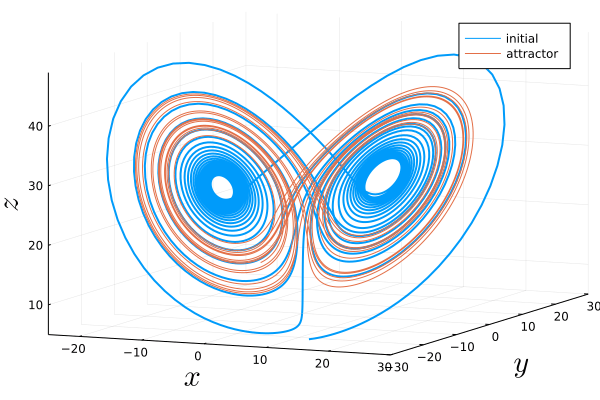
Here, we separated the trajectory in two parts: We plot the initial transient dynamics starting from random initial conditions towards the attractor in blue and the subsequent time evolution lying entirely on the attractor in orange.

Following Refs.⁴ and ⁵, we choose

$$
\langle z \rangle_∞ = \lim_{T \rightarrow ∞} \frac{1}{T} \int_0^T z \text{d}t
$$

as the objective, where we only use the trajectory that lies completely on the attractor (i.e., the orange trajectory in the plot on top). Let us first study the objective as a function of $\rho$.

function compute_objective(sol)
  quadgk(t-> sol(t)[end]/(tspan_attractor[2]-tspan_attractor[1]) ,tspan_attractor[1],tspan_attractor[2], atol=1e-14, rtol=1e-10)[1]
end

pl2 = plot(sol_attractor.t, getindex.(sol_attractor.u,3), ylabel=L"z(t)", xlabel=L"t", label=false, labelfontsize=20,lw = 2)
mean_z = [mean(getindex.(sol_attractor.u,3))]
int_z = compute_objective(sol_attractor)
hline!(pl2, [int_z], label=L"\langle z\rangle", lw = 2)
savefig(pl2, "zsingle.png")

# for each value of the parameter, solve 20 times the initial value problem
# wrap the procedure inside a function depending on p
function Lorenz_solve(p)
  u0 = rand(3)
  prob_init = ODEProblem(lorenz!,u0,tspan_init,p)
  sol_init = solve(prob_init,Tsit5())
  prob_attractor = ODEProblem(lorenz!,sol_init[end],tspan_attractor,p)
  sol_attractor = solve(prob_attractor,Vern9(),abstol=1e-14,reltol=1e-14)
  sol_attractor, prob_attractor
end

Niter = 10
ps = collect(0.0:1.0:50.0)
probs = []
sols = []
zmean = []
zstd = []
for ρ in ps
  @show ρ
  ztmp = []
  for i=1:Niter
    sol, prob = Lorenz_solve([ρ])
    zbar = compute_objective(sol)
    push!(sols, sol)
    push!(probs, prob)
    push!(ztmp, zbar)
  end
  push!(zmean,mean(ztmp))
  push!(zstd,std(ztmp))
end

pl3 = plot(ps,zmean, ribbon = zstd, ylabel=L"\langle z\rangle", xlabel=L"\rho", legend=false, labelfontsize=20, lw = 2, xlims=(0,50),ylims=(0,50))
savefig(pl3, "zvsrho.png")

pl4 = plot(pl2,pl3, margin=3Plots.mm, layout = (1, 2), size=(600,300))
savefig(pl4, "z.png")

We obtain:

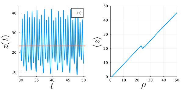
That is, we find a slope of approximately one (almost everywhere except at the kink $\rho\approx 23$), and, therefore, we expect a sensitivity of

$$
\frac{\text{d}\langle z \rangle_∞}{\text{d} \rho} \approx 1.
$$

Conventional forward-mode sensitivity analysis and finite-differencing

For non-chaotic systems, we would just use the
standard discrete or continuous forward sensitivity methods or even finite-differencing. If we try to compute the sensitivity for the Lorenz system:

function G(p, prob=prob_attractor)
  tmp_prob = remake(prob,p=p)
  tmp_sol = solve(tmp_prob,Vern9(),abstol=1e-14,reltol=1e-14)
  res = compute_objective(tmp_sol)
  @info res
  res
end
sense_forward = ForwardDiff.gradient(G,p)
sense_calculus = Calculus.gradient(G,p)

we find diverging values:

$$
\begin{aligned}
& \frac{\text{d}\langle z \rangle_\infty}{\text{d} \rho} \Bigg\rvert_{\rho=28} \approx -49899 {\text{ (ForwardDiff)}} \\
&\frac{\text{d}\langle z \rangle_\infty}{\text{d} \rho} \Bigg\rvert_{\rho=28} \approx 472 {\text{ (Calculus)}}
\end{aligned}
$$

As pointed out in the NILSS paper, this is because the limit of $T\rightarrow ∞$ for a fixed initial state does not commute with the differentiation:

$$
\frac{\text{d}}{\text{d} \rho} \langle z \rangle_∞ \neq \lim_{T \rightarrow ∞} \frac{\partial}{\partial \rho} \langle z \rangle_T
$$

Similarly, using
uncertainty quantification one realizes that due to finite numerical precision and the associated unavoidable errors that are amplified exponentially, one cannot follow the true solution of a chaotic system for long times. We can visualize this by solving the Lorenz system twice with exactly the same parameters and initial condition but with different floating point number precision. In the following animation, we see an $O(1)$ difference between both trajectories after a few Lyapunov lengths:

prob_attractor1 = ODEProblem(lorenz!,sol_init[end],(0.0, 50.0),p)
prob_attractor2 = ODEProblem(lorenz!,convert.(Float32, sol_init[end]),(0f0, 50f0),convert.(Float32,p))
sol1 = solve(prob_attractor1,Tsit5(),abstol=1e-6,reltol=1e-6, saveat=0.01)
sol2 = solve(prob_attractor2,Tsit5(),abstol=1f-6,reltol=1f-6, saveat=0.01f0)

list_plots = []
t1 = 0.0
for i in 1:500
  t2 = i*0.1
  plt1 = plot(sol1, vars=(1,2,3), tspan=(t1,t2), denseplot=true, legend=true,
     label = "Float64", labelfontsize=20, lw = 2,
     xlabel = L"x", ylabel = L"y", zlabel = L"z",
     xlims=(-20,25),ylims=(-28,25),zlims=(5,48))
  plot!(plt1, sol2,vars=(1,2,3), tspan=(t1,t2), denseplot=true, label="Float32",
        xlims=(-20,25),ylims=(-28,25),zlims=(5,48))
  push!(list_plots, plt1)
end

anim = animate(list_plots,every=1)

pl1 = plot(sol1,vars=(1,2,3), legend=true,
  label = "Float64", labelfontsize=20, lw = 2,
  xlabel = L"x", ylabel = L"y", zlabel = L"z",
  xlims=(-20,25),ylims=(-28,25),zlims=(5,48)
 )
plot!(pl1, sol2,vars=(1,2,3), label="Float32", xlims=(-20,25),ylims=(-28,25),zlims=(5,48)
 )

savefig(pl1, "Lorenz_Floats.png")

Without animation:

Luckily, the
shadowing lemma states:

Although a numerically computed chaotic trajectory diverges exponentially from the true trajectory with the same initial coordinates, there exists an errorless trajectory with a slightly different initial condition that stays near (“shadows”) the numerically computed one.

Shadowing methods

The central idea of the shadowing methods is to distill the long-time effect (which actually shifts the attractor) due to a variation of the system parameters (upwards in the $z$-direction with increasing $\rho$ for the Lorenz system) from the transient effect, i.e., the butterfly effect that looks like exponentially diverging trajectories due to variations of the initial conditions. That implies that we aim at finding two trajectories, one with $p$ and one with $p+\delta p$, which do not diverge exponentially from each other (which exist thanks to the shadowing lemma). In this case, their difference will only contain the long-time effect. More details can be found in Refs. ⁴ and ⁵, including a visualization of both effects in Fig. 1 of Ref. ⁵.

LSS and NILSS for the Lorenz system

Switching to LSS or NILSS within the
SciML ecosystem is straightforward by either defining the associated LSS (ForwardLSSProblem or AdjointLSSProblem) or NILSS problem (NILSSProblem) type manually:

# objective
g(u,p,t) = u[end]

####
# LSS
####
lss_problem = ForwardLSSProblem(sol_attractor, ForwardLSS(alpha=DiffEqSensitivity.CosWindowing()), g)
@show shadow_forward(lss_problem) # 1.0095888187322035

lss_problem = ForwardLSSProblem(sol_attractor, ForwardLSS(alpha=DiffEqSensitivity.Cos2Windowing()), g)
@show shadow_forward(lss_problem) # 1.0343951385924328

lss_problem = ForwardLSSProblem(sol_attractor, ForwardLSS(alpha=10.0), g)
@show shadow_forward(lss_problem) # 1.0284286902740765

adjointlss_problem = AdjointLSSProblem(sol_attractor, AdjointLSS(alpha=10.0), g)
@show shadow_adjoint(adjointlss_problem) # 1.028428690274077

or by setting the sensealg= kwarg in solve():

# select via sensealg in solve
using Zygote

function GLSS(p; sensealg=ForwardLSS(), dt=0.01, g=nothing)
  _prob = remake(prob_attractor,p=p)
  _sol = solve(_prob,Vern9(),abstol=1e-14,reltol=1e-14,saveat=dt,sensealg=sensealg, g=g)
  sum(getindex.(_sol.u,3))
end

dp1 = Zygote.gradient((p)->GLSS(p),p) # 0.9694728321500617

Note that we have implemented three different options for forward shadowing with LSS():

• CosWindowing() (default)
• Cos2Windowing()
• time dilation with a factor of $\alpha$.

Additionally, an adjoint implementation AdjointLSS() is available that is particularly recommended for a large number of system parameters. Based on the values computed above, we can easily check that AdjointLSS(alpha=10.0) agrees perfectly with ForwardLSS(alpha=10.0). In all cases considered, we find the expected sensitivity value of $\approx 1$.

However, the use of LSS() is (typically) much more expensive than the use of NILSS(), because LSS() needs to solve a large linear system. This linear system scales with the number of independent variables in the differential equation times the number of time steps and, thus, it can become very large. The computational and memory costs of NILSS() scale with the number of positive (unstable) Lyapunov exponents, since it constrains the optimization problem in the LSS method to its unstable subspace. In many cases, this number is much smaller than the number of independent variables, hence making NILSS() more efficient.

In the NILSS() algorithm, the user can control the number of steps per segment as well as the number of segments.

####
# NILSS
####

# make sure trajectory is fully on the attractor
Random.seed!(1234)
tspan_init = (0.0,100.0)
tspan_attractor = (100.0,120.0)
u0 = rand(3)
prob_init = ODEProblem(lorenz!,u0,tspan_init,p)
sol_init = solve(prob_init,Tsit5())
prob_attractor = ODEProblem(lorenz!,sol_init[end],tspan_attractor,p)

nseg = 100 # number of segments on time interval
nstep = 2001 # number of steps on each segment

nilss_prob = NILSSProblem(prob_attractor, NILSS(nseg, nstep), g)
@show DiffEqSensitivity.shadow_forward(nilss_prob,Tsit5()) # 0.9966924374966089

If the number of segments is chosen too small, a warning is thrown:

nseg = 20 # number of segments on time interval
nstep = 2001 # number of steps on each segment

nilss_prob = NILSSProblem(prob_attractor, NILSS(nseg, nstep), g)
@show DiffEqSensitivity.shadow_forward(nilss_prob,Tsit5()) # 1.0416028730638789

# Warning: Detected a large value of ξ at the beginning of a segment.
# └ @ DiffEqSensitivity ~/.julia/dev/DiffEqSensitivity/src/nilss.jl:474

In the future, we might add an option for the automate control of these variables following the proposal in the NILSS paper⁵.

Outlook

With respect to the shadowing methods for chaotic systems, we are planning to implement further methods, such as

• NILSAS⁶
• FD-NILSS⁷

in the upcoming weeks. For further information and a collection of other methods, the interested reader is invited to track the corresponding
issue in the DiffEqSensitivity.jl package.

If you have any questions or comments, please don’t hesitate to contact me!

---

1. Frank Schäfer, Michal Kloc, et al., Mach. Learn.: Sci. Technol. 1, 035009 (2020). ↩︎

2. Frank Schäfer, Pavel Sekatski, et al., Mach. Learn.: Sci. Technol. 2, 035004 (2021). ↩︎

3. Chris Rackauckas, Yingbo Ma, et al., arXiv preprint arXiv:2001.04385 (2020). ↩︎

4. Qiqi Wang, Rui Hu, et al. J. Comput. Phys 26, 210-224 (2014) ↩︎

5. Angxiu Ni and Qiqi Wang. J. Comput. Phys 347, 56-77 (2017). ↩︎

6. Angxiu Ni and Chaitanya Talnikar, J. Comput. Phys 395, 690-709, (2019) ↩︎

7. Angxiu Ni, Qiqi Wang et al., J. Comput. Phys 394, 615-631 (2019) ↩︎

By: julia on Abel Soares Siqueira

Re-posted from: https://abelsiqueira.com/blog/2021-06-28-migracao-franklin/

Update 2022-12-30: Já não uso mais Franklin.jl.
Há algum tempo o Jekyll tem me dado trabalho. Como não sou usuário de Ruby, volta e meia falta alguma coisa na minha instalação e eu passo horas tentando corrigir o problema pra fazer meu site rodar localmente. Para o CiDAMO, eu considerei o Hugo, já que tem mais suporte e eu não seria a única pessoa a cuidar do site. Já para meu site pessoal, e o site do Julia Smooth Optimizers, resolvi usar Franklin, já que eu quero mais é usar Julia mesmo.