By: Frederik Banning

Re-posted from: https://forem.julialang.org/fbanning/julia-abm-2-work-eat-trade-repeat-3d7l

In agent-based modelling we want to advance our simulation in time and let the agents act in accordance with their plans and schedules. Let’s say we want to simulate five time steps. If you for example already have some experience in NetLogo, you might know that this is very simple to do there.

When using a general purpose programming language like Julia, however, we have to do things through code instead of relying on a ready-made graphical user interface (GUI). So if there are no buttons to click on, how do we do this then? This issue will first generally cover how to advance the model through loops, such that afterwards we can go into detail about the work, eat, and trade processes that all of our agents will face every day. Over its course, we will learn about some built-in functions that might come in handy, how to use conditional logic, and a lot of other things – so let’s jump right in.

Advancing the model

In contrast to NetLogo and other GUI-driven ABM frameworks, Julia requires a bit more manual coding work from us. How exactly our program should process the data and by that advance the state of our model is not controlled via buttons to click on but instead we explicitly define all model functionality by writing executable code. Maybe the simplest imaginable way our model state could be incrementally advanced is via a for-loop:

julia> for step in 1:5
           println(step)
       end
1
2
3
4
5

The loop above looks very simple but already does a few things. We use loops a lot when writing ABMs, therefore we will pick the concept apart and briefly explain the important aspects of them.

• for x in y: This is the start of the loop. The command iterates over each item in the provided iterable y. Basically this can be any collection of items that can return its values one at a time. Like in the example above this could be a range of numbers 1:5 (= one to five in increments of one) or any other iterable like an Array, a Tuple, the key-value pairs of a Dict, et cetera.^[1]
• println(x): This is the heart of our for-loop. It is indented to visually set it apart from the surrounding code. Here we can do whatever we want and it will be repeated as many times as there are elements in y. In our example we call the println function which just prints the value of a given variable to the Julia REPL. Here we also created a temporary local variable x that only exists within the loop and changes its value (but not its name) with every iteration of the for-loop. This allows us to reference the current “state of the loop” and do awesome things with it.
• end: As you already know, this is the Julia keyword that marks the end of the preceding block (e.g. an if-block or a for-loop).

As will often be the case in ABMs, in the above example we have gone through the body of the loop for multiple times. Every time we’ve done something with the available data, i.e. printing the current step. If you’re coming from a NetLogo background, what we’ve did above is comparable to writing the following procedures:

to setup
  reset-ticks
end

to go
  tick
  print ticks
end

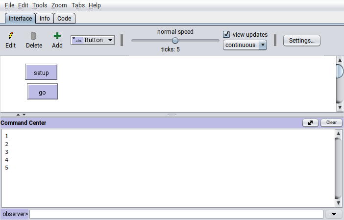
And then setting up the setup and go buttons on the interface, clicking the setup button once and clicking the go button for five times:

Now how to loop over our agents which we’ve stored as separate variables so far? You might have already guessed it: We just store them in a Vector.^[2]

julia> agents = [sally, richard]
2-element Vector{Agent}:
 Agent("Baker", 10, 10, 0, 0)
 Agent("Fisher", 10, 10, 0, 0)

julia> for agent in agents
           println(agent.job)
       end
Baker
Fisher

It’s also possible to not only retrieve agent data inside such loops but we can of course also include some conditional logic statements in there according to which we will alter the agent variables.

julia> for agent in agents
           if agent.job == "Baker"
               println("Sally's oven exploded and burnt down her whole pantry.")
               agent.pantry_bread = 0
               agent.pantry_fish = 0
           elseif agent.job == "Fisher"
               println("Richard was very fortunate today and caught ten fish!")
               agent.pantry_fish += 10
           end
       end
Sally's oven exploded and burnt down her whole pantry.
Richard was very fortunate today and caught ten fish!

The Julia REPL threw back both cases that we’ve included in our loop. The order by which these events are happening is determined by the order of Agents in our collection agents. The new values are saved as the agent variables , i.e. the fields of the two instances of our composite type.

julia> sally
Agent("Baker", 0, 0, 0, 0)

julia> richard
Agent("Fisher", 20, 10, 0, 0)

Of course this was just an illustrative example of what would be possible inside such a loop. But now that we’ve established how to programmatically let our agents experience events and how to change their variables in reaction to these events, we can reason about what they should do each day and build a proper loop for our model.

Work, eat, trade, repeat

While Richard and Sally spend their time on very different things each day, the fundamental steps are still similar: Every day they go after their respective work which makes them hungry so they have to eat. Every third day, they meet to trade fish and bread with each other. The following subsections are about representing these actions as the core loops of our model and describing them in a bit more detail. We’ll start with a simplified version but in later issues we will go on and expand it to be a bit more sophisticated.

Work

As described in our model description, Richard has a chance to catch 0-3 fish per hour that he is out on the sea fishing. Because it would take a lot of time and effort to model the ecosystem of the sea and coastal area that he regularly goes to for fishing, we will opt for a stochastic approach to model his hourly fishing success. This can be easily done in Julia with the built-in rand function. If we don’t pass any arguments to it, it will just provide us with a random floating point number which was drawn from a uniform distribution between 0 and 1

$x\sim U(0,1)$

:

julia> rand()
0.21528920784298688

However, rand is the standard Julia interface for drawing a random element out of a given collection. This means that there are specialised methods for a lot of different use cases, which makes it simple for us to model randomised processes.

julia> rand(1:10)
6

julia> rand(["bark", "meow", "moo"])
"bark"

julia> rand(agents)
Agent("Baker", 10, 10, 0, 0)

Following this logic, we can define a simple list with numbers from 0-3 where the number of occurrences of each number then reflects the probability to draw it randomly.

julia> fishing_chances = [0, 0, 0, 0, 1, 1, 1, 2, 2, 3]
10-element Vector{Int64}:
 0
 0
 0
 0
 1
 1
 1
 2
 2
 3

Since Richard regularly doesn’t go fishing for only one hour but for a few hours at once, it would be nice if we could just make multiple draws from the distribution and sum up those numbers to find out how many fish Richard has caught this day. This is also possible with the rand function when we provide it with the amount of independent draws that we want to make. Let’s say Richard goes fishing for five hours.

julia> fish_per_hour = rand(fishing_chances, 5)
5-element Vector{Int64}:
 0
 0
 0
 1
 0

As you can see we have stored the resulting Vector{Int64} (i.e. a list of integer numbers) in a new variable called fish_per_hour. This not only allows us to find out how many fish he caught during which hour (e.g. the fourth hour) …

julia> fish_per_hour[4]
1

… but it also lets us easily calculate the total amount of caught fish via the sum function.

julia> sum(fish_per_hour)
1

Poor Richard. He went out fishing for five hours and only got one meager fish for all that effort.

The amount of hours he is out on the sea might depend on things like how filled his pantry currently is, how many fish he tries to set aside for Sally, and his previous luck during this day. Since some of these things depend on the other two core processes “eat” and “trade” which we will discuss further down, we can just currently assume that his daily fishing efforts depend on a random draw from a uniform distribution

$\text{fishing hours}\sim U(1,5)$

as well.

Julia allows us to nest one call to a function into another and by that use the result of the inner call as input for the outer call. This may sound a bit complicated at first but is easy to demonstrate and even easier to intuitively understand when you see the results:

julia> rand(fishing_chances, rand(1:5))
1-element Vector{Int64}:
 3

julia> rand(fishing_chances, rand(1:5))
2-element Vector{Int64}:
 2
 0

The second result reads as follows: Richard went fishing for two hours (the length of the Vector). He caught two fish in the first hour and not a single one in the second hour (the elements of the Vector). Overall he caught two fish which means that he caught one fish per hour on average (the sum and mean of the Vector).

Richard spends the remainder of his work day on various other tasks. Again, this might depend on various factors but for now we will just assume that he works for at least one more hour and up to three hours after returning from sea. Can you guess how we will do this? (Hint: It may or may not have something to do with the rand function.)

Determine other work hours (click me)

rand(1:3)

Lucky for Sally that she’s not so dependent on the whims of the sea but can freely decide to produce up to 20 loaves of bread each day. How many she wants to bake may depend on various factors, just like it is the case for Richard’s fishing endeavours. For example, her current and future hunger levels, how many loaves she needs for trading with Richard, or maybe just her motivation on that day might factor into her decision. But we do not have all this information at the current stage and can only add these ideas later. So for now, we will also just make a simplifying assumption to randomise the amount of freshly baked bread as

$\text{fresh bread}\sim U(1,20)$

:

julia> rand(1:20)
15

During this day, Sally decided to bake 15 loaves of bread. As we know, she needs to work for at least eight hours even if she only bakes a single bread. But baking the maximum of 20 loaves will only take up 10 hours in total, so the increase in necessary working time per additional bread is quite small. How small exactly is something that we can find out with just a single Julia command again.

julia> hours_for_breads = LinRange(8, 10, 20)
20-element LinRange{Float64, Int64}:
 8.0,8.10526,8.21053,8.31579,8.42105,8.52632,8.63158,8.73684,…,9.36842,9.47368,9.57895,9.68421,9.78947,9.89474,10.0

LinRange takes a starting number (8), an ending number (10), and the length (20) of the resulting range. From this range of numbers with equal distance between them (LinRange stands for “linear range”) we can now deduct how many hours Sally had to work to bake 15 fresh loaves of bread.

julia> hours_for_breads[15]
9.473684210526315

Great! So far we have established two simple algorithms to find out how many hours Sally and Richard work on a day and what the fruit of their labour might look like. Now let’s combine the above-mentioned processes into a single for-loop, just how we learned it at the beginning of this post.

for agent in agents
    if agent.job == "Baker"
        # bake bread and add to pantry
    elseif agent.job == "Fisher"
        # go fishing and add to pantry
    end
end

Can you finish this piece of code? Look at the explanations above and try it out by yourself.

Remember that you can add temporary variables like hours_for_breads to make it easier to reason about the flow of the code. If you prefer to write your code in a less verbose way, you can also opt for nesting function calls into each other, thus reducing the lines of code that you have to write. A word of warning though:

It is often better to be as explicit as possible about what you intend your code to do.
This is especially true if you want other people to read and understand your code but is just as important for your future self.

• Pick “telling names” for your variables.
• Stick to a coherent coding style.
• Find the right balance between verbosity and conciseness.

Verbose & concise solutions (click me)

# verbose version with comments for individual subprocesses
for agent in agents
    if agent.job == "Baker"
        # determine how many loaves of bread Sally will bake this day
        fresh_breads = rand(1:20)
        # add freshly baked bread to Sally's pantry
        agent.pantry_bread += fresh_breads
        # get a list of working hours required to bake a certain amount of bread
        hours_for_breads = LinRange(8, 10, 20)
        # find out how many hours Sally needs to work for this
        baking_hours = hours_for_breads[fresh_breads]
    elseif agent.job == "Fisher"
        # make a random draw for Richard's fishing hours
        fishing_hours = rand(1:5)
        # create an array to represent the probability to catch fish
        fishing_chances = [0, 0, 0, 0, 1, 1, 1, 2, 2, 3]
        # make `fishing_hours` random draws from `fishing_chances` to get a list of fish per hour
        fresh_fish = rand(fishing_chances, fishing_hours)
        # add freshly caught fish to Richard's pantry
        agent.pantry_fish += sum(fresh_fish)
        # randomly determine the rest of Richard's working hours for tasks other than fishing
        other_work_hours = rand(1:3)
    end
end

# concise version with nesting and without comments
for agent in agents
    if agent.job == "Baker"
        fresh_breads = rand(1:20)
        agent.pantry_bread += fresh_breads
        baking_hours = LinRange(8, 10, 20)[fresh_breads]
    elseif agent.job == "Fisher"
        fishing_hours = rand(1:5)
        fresh_fish = rand([0, 0, 0, 0, 1, 1, 1, 2, 2, 3], fishing_hours)
        agent.pantry_fish += sum(fresh_fish)
        other_work_hours = rand(1:3)
    end
end

Eat

When our agents work, they get hungry and need to eat. In this respect, we will again start simple and say that both Sally and Richard need one loaf of bread (1 kg) and half a fish (0.5 kg) each day. With our newfound power of iteration via for-loops, we can do that for all our agents in one go:

julia> for agent in agents
           agent.hunger_bread += 1
           agent.hunger_fish += 0.5
       end
ERROR: InexactError: Int64(0.5)
Stacktrace:
 [1] Int64
   @ ./float.jl:812 [inlined]
 [2] convert
   @ ./number.jl:7 [inlined]
 [3] setproperty!(x::Agent, f::Symbol, v::Float64)
   @ Base ./Base.jl:43
 [4] top-level scope
   @ ./REPL[23]:3

Wait, we seem to not have anticipated that our agents might not always want to eat a whole fish or loaf of bread at once. We just tried to account for fractions of fish but our struct only allows for whole units of bread and fish because we chose Int as an inappropriate type for the pantry fields. Throwing away the rest of the fish is also not an option because it would be both very wasteful and disrespectful towards the animal.

Luckily the stacktrace (that’s the menacing looking message that Julia throws at us when there’s an error) tells us that it cannot convert the number 0.5 into an Int64.^[3] It also tells us that it tried to set the agent variable to a Float64 (see [3] in the stacktrace). With this information, it’s easy to fix this small oversight from our preliminary modelling process by redefining our custom-made composite type Agent. The new struct should now look like this:

julia> mutable struct Agent
           job::String
           pantry_fish::Float64
           pantry_bread::Float64
           hunger_fish::Float64
           hunger_bread::Float64
       end

The new types of the fields are 64 bit floating point numbers, which are called Float64 in Julia, and are able to represent fractions of something as a number. If we’re talking about our food in terms of kilograms, then in our case an agent is now able to store half a kilo of bread via pantry_bread += 0.5 or represent their craving for half a pound of fish by setting hunger_fish = 0.25.

After redefining sally and richard with our freshly adjusted Agent struct and placing them in the list of agents, we can run the loop from above again:

julia> for agent in agents
           agent.hunger_bread += 1
           agent.hunger_fish += 0.5
       end

julia> agents
2-element Vector{Agent}:
 Agent("Baker", 10.0, 10.0, 0.5, 1.0)
 Agent("Fisher", 10.0, 10.0, 0.5, 1.0)

Et voilà, it worked just as expected. Naturally, the next step is about satisfying their hunger by eating something. This is in fact just as simple to code as the loop before. We subtract the amount of food to eat from the pantry and reduce the hunger level for it during:

julia> for agent in agents
           agent.pantry_bread -= 1.0
           agent.hunger_bread -= 1.0
           agent.pantry_fish -= 0.5
           agent.hunger_fish -= 0.5
       end

julia> agents
2-element Vector{Agent}:
 Agent("Baker", 9.5, 9.0, 0.0, 0.0)
 Agent("Fisher", 9.5, 9.0, 0.0, 0.0)

Now as a thought experiment, we could try to run this loop again. Don’t actually do it but instead try to reason about what you think will happen?

New state of agent variables (click me)

julia> agents
2-element Vector{Agent}:
 Agent("Baker", 9.0, 8.0, -0.5, -1.0)
 Agent("Fisher", 9.0, 8.0, -0.5, -1.0)

The amount of fish and bread in the pantry was reduced by the correct amount but the hunger levels of our agents became negative. The phenomenon of overeating is undoubtably a thing in real life but we do not want to include it in our model as it might conflict with our modelling question and would require further assumptions to make it believable.

To avoid negative hunger levels, we need to introduce a bit of conditional logic (if, elseif, else) in our loop to make sure that our agents only eat (i) as much as they need and (ii) as much as they have. We can account for these two conditions in two different ways:

julia> for agent in agents
           # completely satisfy hunger when there's enough food in pantry
           if agent.pantry_fish >= agent.hunger_fish
               agent.pantry_fish -= agent.hunger_fish
               agent.hunger_fish = 0
           end
           if agent.pantry_bread >= agent.hunger_bread
               agent.pantry_bread -= agent.hunger_bread
               agent.hunger_bread = 0
           end

           # partially satisfy hunger until pantry is empty
           if 0 < agent.pantry_fish <= agent.hunger_fish
               agent.hunger_fish -= agent.pantry_fish
               agent.pantry_fish = 0
           end
           if 0 < agent.pantry_bread <= agent.hunger_bread
               agent.hunger_bread -= agent.pantry_bread
               agent.pantry_bread = 0
           end
       end

Well, look at that. This is already quite nice! So far we’ve captured the fundamental concepts of working, getting hungry, and eating, all while keeping stock of the available food for each agent.

At some point, however, our agents will find themselves in a bit of a pickle: Sally the baker will run out of fish and Richard the fisher will run out of bread. Humans are great at cooperating with each other to fulfil their own needs. So in the next step, we will introduce a basic system of trade between our two hardworking agents.

Trade

On every third day, our two friends meet up at the oceanside for a nightcap and to exchange their produce with each other. According to how we currently modelled daily increases in hunger levels, both agents know that they need 3 bread and 1.5 fish for the timespan of three days, so that’s certainly the minimum of food that they want to have in their pantry after trading with each other. We will stick to our initial assumption for now and say that these trades are happening at a one to one ratio. Furthermore, we assume that they will not reserve any of their produce for themselves but are willing to trade as much with the other agent as they want or as they themselves have available.

In contrast to how we modelled working and eating before, we are not going to iterate over all agents this time around. Instead we know that bilateral trade happens between pairs of interacting agents and since we only have two agents in our little world, things are getting a bit easier to handle. We can just use the agents’ variable names sally and richard again to access and change their data. Don’t worry, the new values will automatically be reflected in the agents Vector as well.

For any trading to happen, we need to make sure that a few conditions apply:

1. Sally has any bread and Richard has any fish.
2. Sally has less than 1.5 fish in her pantry.
3. Richard has less than 3 bread in his pantry.

Trading shall only cover the minimum amount of bread/fish that are needed and affordable by Sally and Richard while at the same time being available from the other agent.

To achieve this, we use the built-in min function which returns the minimum value of the arguments we pass to it. With it, we account for the three different limiting factors, namely the agent’s needs (want), their own available goods for trade (affordability), or their trade partner’s available goods (availability). Once we’ve determined from this that a trade happens and how many goods are traded, we can put the pieces together such that the algorithm for the trading in our model currently looks like this:

if sally.pantry_fish < 1.5
    sally_wants_fish = 1.5 - sally.pantry_fish
    traded_fish = min(sally_wants_fish, sally.pantry_bread, richard.pantry_fish)
    # trade ratio of 1:1 means that the amounts of traded fish and bread are equal
    traded_bread = traded_fish

    sally.pantry_bread -= traded_bread
    sally.pantry_fish += traded_fish
    richard.pantry_fish -= traded_fish
    richard.pantry_bread += traded_bread
end

if richard.pantry_bread < 3.0
    richard_wants_bread = 3.0 - richard.pantry_bread
    traded_bread = min(richard_wants_bread, sally.pantry_bread, richard.pantry_fish)
    traded_fish = traded_bread

    sally.pantry_bread -= traded_bread
    sally.pantry_fish += traded_fish
    richard.pantry_fish -= traded_fish
    richard.pantry_bread += traded_bread
end

What this sequence mimics, is the process of Sally first determining how many fish she lacks, then asking for a few fish from Richard up until either him or her do not have any more resources to trade. After this first round of trading, Richard checks if he now already has enough bread in his pantry. When that isn’t the case, he asks Sally for the remaining necessary loaves.

After we’ve figured out how to put this straight-forward trading into code, we will start to balance things out by adjusting the ratio at which the two goods are traded. Since the regular need for bread is twice as high as that for fish, we will now assume a new trading ratio of one fish to two loaves of bread (in other words: one fish is worth twice as much as one bread). Formalising this takes only very slightly more effort from our side to account for the newly introduced ratio’s influence on the limiting factors:

if sally.pantry_fish < 1.5
    sally_wants_fish = 1.5 - sally.pantry_fish
    traded_fish = min(sally_wants_fish, sally.pantry_bread / 2, richard.pantry_fish)
    traded_bread = 2 * traded_fish

    sally.pantry_bread -= traded_bread
    sally.pantry_fish += traded_fish
    richard.pantry_fish -= traded_fish
    richard.pantry_bread += traded_bread
    end
end

if richard.pantry_bread < 3.0
    richard_wants_bread = 3.0 - richard.pantry_bread
    traded_bread = min(richard_wants_bread, sally.pantry_bread, richard.pantry_fish * 2)
    traded_fish = traded_bread / 2

    sally.pantry_bread -= traded_bread
    sally.pantry_fish += traded_fish
    richard.pantry_fish -= traded_fish
    richard.pantry_bread += traded_bread
end

And as easy as that we have created a fundamental trading process that allows our agents to exchange their produce with each other.

Summary and outlook

In this issue of the “Julia ♥ ABM” series, we have learned a lot of fundamentally important things for creating ABMs in Julia, specifically how to…

• advance our model with for-loops,
• iterate over agents to access and change their variables,
• make random draws with the built-in rand function,
• create a linear range of numbers with equal distance between its steps,
• not panic when encountering an error message and instead use the provided information to our advantage,
• use logic statements to control the flow of our model, and
• find the minimum of a given set of numbers with the built-in min function.

That’s already quite a lot to take in at once, so we will leave it here for the time being. In the next issue, we make the work, eat, and trade subprocesses resuable by encapsulating them in functions and continue by bundling subprocesses into one cohesive loop representing a day in the life of our agents.

[1]: Interested in learning a bit more about what you can do with collections in Julia? Have a look at the section on collections in the Julia docs and specifically also at the subsection on iterable collections. But to be quite frank, Julia doesn’t really do anything special when it comes to dealing with iterables, so it’s likely able to do everything you would expect it to. This means that, among a lot of other things, you could collect only unique items, find their extrema, and reduce the collection via a binary operator.

[2]: A Vector is a specialised form of an Array which has just one dimension. Generally speaking, Vectors are subtypes of Arrays:

julia> Vector <: Array
true

julia> Vector{Int} <: Array{Int, 1}
true

which means that all the methods that work on Arrays will also work on Vectors but not necessarily vice versa. This is quite nice for us because we can be pretty sure that the interface to interact with an Array will be the same across its subtypes. This relieves us of a bit of mental burden when it comes to how to interact with various types. A Matrix, for example, is a multi-dimensional Array and we can retrieve its size in exactly the same way as we would do it for a Vector.

julia> v = [1, 2, 3]
3-element Vector{Int64}:
 1
 2
 3

julia> size(v)
(3,)

julia> a = [[1, 2, 3] [4, 5, 6]]
3×2 Matrix{Int64}:
 1  4
 2  5
 3  6

julia> size(a)
(3, 2)

We’ve already briefly talked about Julia’s typing system in Issue 1, so if you’ve missed or skipped that piece of information, feel free to check back there and read up on the basics.

[3]: There are quite a lot of different types of errors that Julia can confront us with. In this specific case, it was an InexactError which tells us that there is not an exact way to represent a fraction 1/2 or a decimal number 0.5 as an integer number. Other types of errors that you are very likely to encounter over the course of your Julia journey are UndefVarError (trying to reference a variable before defining it), MethodError (trying to use a function that is lacking a specific method for the combination of arguments that you passed), UndefKeywordError (trying to use a function which requires you to specify a value for one of its keyword arguments), and many more. If you’re interested in learning more about these, the Julia documentation also has a short section on errors and how to work with them.