Category Archives: Julia

DataFrames.jl survey: selecting columns of a data frame based on their values

By: Blog by Bogumił Kamiński

Re-posted from: https://bkamins.github.io/julialang/2023/08/18/selectcolumn.html

Introduction

Today I want to make a user survey about a future direction
of development of DataFrames.jl.

Most commonly users want to select columns of a data frame
using their names and this is the operation that has an
extensive support in DataFrames.jl.
However, in some cases one might need to perform such a
selection conditional on a value stored in a column.

I want to ask if we should add a special selector allowing for
picking columns of a data frame based on their values.
The question is given in the conclusions section.
However, before we get to it let us briefly review what is
currently supported.

The post was written using Julia 1.9.2 and DataFrames.jl 1.6.1.

Column selection using column names

First create a simple data frame on which we are going
to perform the column selection examples:

julia> using DataFrames

julia> df = DataFrame(a1 = [1, 2],
                      a2=[1, missing],
                      b1=Any[3, missing],
                      b2=Any[3, 4])
2×4 DataFrame
 Row │ a1     a2       b1       b2
     │ Int64  Int64?   Any      Any
─────┼──────────────────────────────
   1 │     1        1  3        3
   2 │     2  missing  missing  4

Now assume we want to pick columns whose name starts with "b":

julia> select(df, Cols(startswith("b")))
2×2 DataFrame
 Row │ b1       b2
     │ Any      Any
─────┼──────────────
   1 │ 3        3
   2 │ missing  4

As you can see, if you pass a function returning a Bool
(such a function is often called a predicate) to Cols
selector you get columns whose names math the condition
defined by this function.

Today I want to focus on cases when you specify the condition
using a function. However, let me mention that there
are other ways to perform selection we discussed above. For example
we could use a regular expression:

julia> select(df, Cols(r"^b"))
2×2 DataFrame
 Row │ b1       b2
     │ Any      Any
─────┼──────────────
   1 │ 3        3
   2 │ missing  4

In general, in DataFrames.jl you currently have the following ways to
select columns (Warning! The list is long.):

  • a symbol, string, or integer;
  • vector of symbols, strings, integers, or bools;
  • regular expression;
  • All, Between, Cols, Not, and : selectors.

Column selection using column values

What if we wanted to select the columns using their values.
For example, assume that we want to pick columns that contain
missing value. In this case the easiest way to do it is to
use the eachcol(df) iterator over columns of our data frame:

julia> select(df, any.(ismissing, eachcol(df)))
2×2 DataFrame
 Row │ a2       b1
     │ Int64?   Any
─────┼──────────────────
   1 │       1  3
   2 │ missing  missing

Notice that the any.(ismissing, eachcol(df)) condition
iterates all columns of df and for each of them returns true
if they contain any missing value (and false otherwise):

julia> any.(ismissing, eachcol(df))
4-element BitVector:
 0
 1
 1
 0

An alternative, similar condition would be to select all columns
that allow for storing missing value (without requiring that
they actually have it stored in them). For this we need to use
the eltype function on columns:

julia> select(df, Missing .<: eltype.(eachcol(df)))
2×3 DataFrame
 Row │ a2       b1       b2
     │ Int64?   Any      Any
─────┼───────────────────────
   1 │       1  3        3
   2 │ missing  missing  4

Note that the difference is column :b2, which does not
contain missing values, but could contain them since its
element type is Any.

Column selection using column names and values

Now, what if we wanted to perform column selection based on both
their names and values?

The general pattern uses pairs(eachcol(df)) which iterates
pairs of column names and values:

julia> pairs(eachcol(df))
Iterators.Pairs(::DataFrames.DataFrameColumns{DataFrame}, ::Vector{Symbol})(...):
  :a1 => [1, 2]
  :a2 => Union{Missing, Int64}[1, missing]
  :b1 => Any[3, missing]
  :b2 => Any[3, 4]

So for example if we wanted to pick columns that contain missing values
and start with "a" we can write:

julia> select(df, [startswith(string(n), "a") && any(ismissing, c)
                   for (n,c) in pairs(eachcol(df))])
2×1 DataFrame
 Row │ a2
     │ Int64?
─────┼─────────
   1 │       1
   2 │ missing

This pattern is fully general, but slightly verbose, especially column names
returned by pairs are Symbols. The same condition
can be written more naturally as follows:

julia> select(df, Cols(startswith("a"),
                       any.(ismissing, eachcol(df));
                       operator=intersect))
2×1 DataFrame
 Row │ a2
     │ Int64?
─────┼─────────
   1 │       1
   2 │ missing

Here we take advantage of the fact that our condition was a conjunction
and Cols selector accepts the operator keyword argument with allows
to get an intersection of two selectors.

If we wanted to select columns that meet
at least one of the conditions this would be even simpler:

julia> select(df, Cols(startswith("a"),
                       any.(ismissing, eachcol(df))))
2×3 DataFrame
 Row │ a1     a2       b1
     │ Int64  Int64?   Any
─────┼─────────────────────────
   1 │     1        1  3
   2 │     2  missing  missing

Note that by default Cols select columns that are a union of selectors
passed to it.

Conclusions

I hope the examples I presented today will be useful when you work with
DataFrames.jl.

You might ask why, when performing column selection
based on their values one needs to invoke eachcol(df). This is indeed
a bit verbose. However, we decided that Cols(predicate), which is
shorter to write should apply the predicate function to column names
as this is a more common operation. And if user wants to apply
the predicate function to column values (which is a less frequent case)
writing predicate.(eachcol(df)) is readable and easy enough.

If we added a built-in way for selection of columns by value
it would mean that instead of writing
predicate.(eachcol(df)) you would write something like
Vals(predicate) (the Vals is an example name – the choice of name can
be done later).

The benefits of having it are:

  • It is shorter.
  • We do not have a redundance of having to pass the df data frame in the expression.

Here are the cons of adding it:

  • It makes the list of things to learn longer (and the list is already quite long).
  • It is ambiguous how the Vals(predicate) should be interpreted if it were
    used in the context of GroupedDataFrame as the question would be how should we
    treat the groups (so most likely it should be only allowed for AbstractDataFrame).
  • It would require a change of internal memory layout of DataFrame object
    (which means that the next release of DataFrames.jl would be incompatible on
    binary level with the current release so serialization/deserialization would
    not work cross-versions).

Now comes the question:

Should we add a new special selector that would allow picking
columns based on their values?

If you have an opinion please vote or comment in this issue on GitHub.

Pythagorean Triples with Comprehensions

By: Jonathan Carroll

Re-posted from: https://jcarroll.com.au/2023/08/13/pythagorean-triples-with-comprehensions/

I’ve been learning at least one new programming language per month through Exercism and the #12in23 challenge. I’ve keep saying,
every time you learn a new language, you learn something about all the others
you know. Plus, once you know \(N\) languages, the \(N+1^{\rm th}\) is significantly easier. This
post covers a calculation I came across in Haskell, and how I can now do the same
in a lot of other languages – and perhaps can’t as easily in others.

All of the languages here, I’m learning via Exercism, or at least I’m completing
a handful or more exercises in each of the languages, which means learning enough
of the syntax to be able to complete those. The #12in23 challenge is to
try 12 languages in 2023… I’m doing just fine so far

#12in23 progress as of July 2023 - I already have my 12, but no reason to stop now

#12in23 progress as of July 2023 – I already have my 12, but no reason to stop now

Haskell

I’ve been reading the (great!) online version of Learn You a Haskell for Great Good! – Haskell is a (properly) “pure” functional
language, part of which means it has no side-effects, which includes, say,
printing to the console. Haskell, of course, has a way around this (monads!) but
it means there’s a lot to get through before you even get to a printing “Hello, World!”
example. It’s also lazy which means it doesn’t evaluate something if it doesn’t
need to, which makes for some good performance, sometimes.

This video does a really nice job explaining the
principles of pure functional programming using JavaScript to introduce Haskell,
building recursive functions that only take a single argument and return a
single value.

One example that caught my eye in the list comprehensions section was this

ghci> let rightTriangles' = [ (a,b,c) | c <- [1..10], b <- [1..c], a <- [1..b], a^2 + b^2 == c^2, a+b+c == 24]  
ghci> rightTriangles'  
[(6,8,10)]  

This perhaps isn’t too hard to read, even for those unfamiliar with the language. ghci is
the interactive REPL for the Glasgow Haskell Compiler, so the prompt starts with that.
Haskell uses a let binding to identify variables, and the apostrophe just indicates that
this is a slightly different version compared to the one defined slightly earlier in the chapter.

The list comprehension itself is perhaps not so dissimilar to one you’d find in Python; it
defines some tuple (a, b, c) and | identifies some constraints, namely that c is taken
from a range of 1 to 10, b is taken from a range of 1 to c, and a is taken from
a range of 1 to b, along with the criteria that \(a^2 + b^2 = c^2\) (the numbers form a Pythagorean
triple) and their sum is 24. I discussed the Pythagorean triples in my last post – no
coincidence (/s). If you evaluate this line, you more-or-less immediately get back the result

[(6,8,10)]

which is a Pythagorean triple

\[6^2 + 8^2 = 36 + 64 = 100 = 10^2\]

for which

\[a + b + c = 6 + 8 + 10 = 24\]
This isn’t a groundbreaking calculation, but I’ve done a lot of R, and my mind
was a little blown that such a calculation could really be done in a single line just
by specifying those constraints. Not a solver, not a grid of values with a filter, just
specifying constraints.

R

Anyone who knows me knows I write a lot of R. I wrote a book on it. I solved all of the
Advent of Code 2022 puzzles in strictly base R (I really need to write that post).

Now, R (unfortunately) doesn’t have any comprehensions, list or otherwise, so I started to
wonder how I would do this in R. The best I can come up with is

expand.grid(a=1:10, b=1:10, c=1:10) |>
  dplyr::filter(a^2 + b^2 == c^2 & 
                  a + b + c == 24 & 
                  a < b & 
                  b < c)
##   a b  c
## 1 6 8 10

but that involves explicitly creating all 1000 combinations of a, b, and c. There
may be a multi-step way to limit the grid to \(a < b\) and \(b < c\) but that’s more code. Maybe the
Haskell solution also has to generate these behind the scenes, but it isn’t up to the user to
do that, so it feels nicer. I like the filter() verb here – technically the & joining is
redundant and I could have passed each condition as its own argument. expand.grid() is one
of those underutilised functions that comes in very handy sometimes – or its cousin
tidyr::crossing() which wraps this and additionally performs de-duplication and sorting.

Now that I know more languages, I felt I could explore this a bit further!

Python

In Python, which I feel is well-known for list comprehensions, this translates more
or less 1:1 to

[(a,b,c) for c in range(1,11) for b in range(1,c) for a in range(1,b) if ((a**2 + b**2) == c**2) if a+b+c==24]
[(6, 8, 10)]

Of course, ranges are specified differently, but otherwise this follows the Haskell
solution quite nicely, including the dynamic ranges of b and a which avoids needing
to search the entire 10*10*10 space.

I appreciate there’s a silly language war between Python and R but
honestly, a lot of stuff is written in Python and a lot of people write in Python.
I figure it’s better to understand that language for when I need it than to stick my
head in the sand and claim some sort of superiority. There’s bits I don’t like, sure,
but that doesn’t mean I shouldn’t learn it. I’m even registered and attending PyConAU next
weekend.

Rust

Rust is a fun language with easily the most helpful compiler ever made – you can make a
lot of mistakes, but the error messages and hints are unparalleled. I’m currently
taking Tim McNamara’s ‘How To Learn Rust’ course which has a
lot of practical lessons and I’ve built some fun things already. I completed the first 13 Advent of Code 2022 puzzles in Rust, after which it all
got a bit too complicated (and I do really need to write that post).

Rust doesn’t have list comprehensions (I believe there are cargo crates which do add
such functionality) so it’s back to nested loops

for c in 1..=10 {
  for b in 1..=c {
    for a in 1..=b {
      if a*a + b*b == c*c && a+b+c == 24 {
        println!("{}, {}, {}", a, b, c);
      }
    }
  }
};
6, 8, 10

That doesn’t allocate a result at all, it just prints the values when it
encounters them, and since the loop is nested, it can limit the search to \(b \leq c\) and
\(a \leq b\), but it does explicitly run the loop across all those combinations. It’s
possible there’s a much better way to do this, but I couldn’t think of it.

Common Lisp

I like the idea of Common Lisp, and I’m making my way through Practical Common Lisp slowly. I suspect I enjoy some of the descendants
like Clojure a bit more, but it’s absolutely worth learning. Miles McBain has a great post
about how learning about lisp quoting helps understand more of the tidyverse. I have used
lisp in a code-golf post.

Lisp doesn’t have comprehensions so it relies on loops, and again, just prints the
result, returning NIL

  (loop for c from 1 to 10
        do (loop for b from 1 to c
                 do (loop for a from 1 to b
                      do (when (and (= (+ a b c) 24) (= (+ (* a a) (* b b)) (* c c)))
                        (format t "~d, ~d, ~d~%" a b c)))))
6, 8, 10
NIL

The loop is still constrained to \(b \leq c\) and \(a \leq b\), but definitely runs
through all those values.

Julia

I really want to learn more Julia, but I’m not entirely new to the language. I have completed
the first 25 Project Euler problems in Julia (by
no means optimised solutions). I think what’s holding me back is the fact that almost
every presentation using it is so very mathsy – and I’m a physicist by training. I love
that the tidyverse is making its way over in the forms of Queryverse,
DataFramesMeta, and more recently (and
most likely with more success) the Tidier family.

Julia does have list comprehensions, and additionally has an “element” operator with
the mathematically-familiar symbol

[(a,b,c) for c ∈ 1:10, b ∈ 1:10, a ∈ 1:10 if (a^2 + b^2 == c^2) && (a+b+c == 24) && b <= c && a <= b]
1-element Vector{Tuple{Int64, Int64, Int64}}:
 (6, 8, 10)

Unfortunately, the choices for b and a still need to run through all 10 values because
Julia doesn’t allow these to be co-defined like Haskell and Python do. I came to Julia from
mainly only knowing R, so dealing with an output of type Vector{Tuple{Int64, Int64, Int64}}
initially proved to be a challenge, but I’d say learning more Rust has made me feel a lot more
comfortable around working with types.

Clojure

Clojure feels to me like “lisp, but with good libraries”. There’s definitely syntax
differences, but most of them feel like improvements.

(for [c (range 11)
      b (range c)
      a (range b)
     :when (and (== (+ (* a a) (* b b)) (* c c)) (== (+ a b c) 24))]
[a b c])
([6 8 10])

This still feels like a comprehension, but the syntax is certainly a bit more
convoluted. Bonus points for the dynamic ranges of b and a. Still, a long way
off of completely unreadable, I’d say.

Scala

I’m learning a lot of functional programming, and I think I’m happy that some of the
textbooks use Scala rather than some alternatives. I’m still very new to this language,
but so far I think I like it.

Again, we’re back to a loop, but most of it is straightforward assignments and we
get the dynamic ranges of b and a

for {
     c <- 1 until 11
     b <- 1 until c
     a <- 1 until b
     if a * a + b * b == c * c & a + b + c == 24
     } {
        println(s"Side lengths: $a, $b, $c")
}
Side lengths: 6, 8, 10

C

I mentioned that I performed this calculation in C in my last post – that
ends up being just a loop

int a, b, c

printf("%4s\t%4s\t%4s\t%4s\n", "a", "b", "c");
printf("   -------------------------\n");
for (c = 1; c <= 24; c++) 
  for (b = 1; b <= c; b++)
    for (a = 1; a <= b; a++)
      if ( ( pow ( a, 2 ) + pow ( b, 2 ) ) == pow ( c, 2 ) ) {
        printf("%4i\t%4i\t%4i\t%4i\n", a, b, c);
      }

I haven’t run the output directly, since it needs an entire program supporting it, but
it’s the right answer.


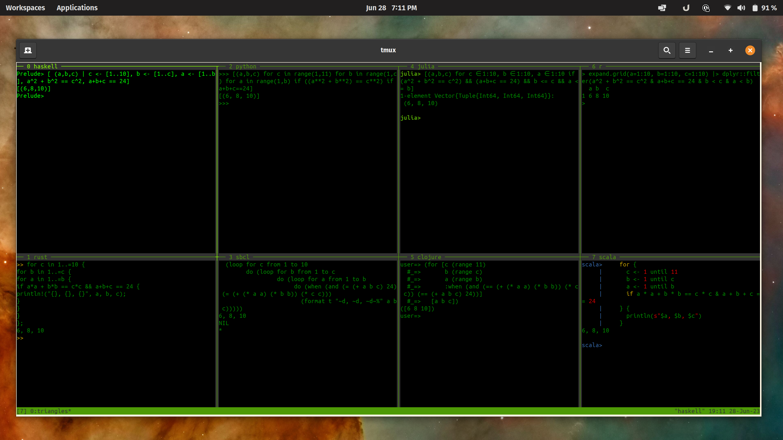
So, what does it look like if you run all of these together? I’ve been getting back
into using tmux and it’s very powerful. One of the
features is splitting a window into panes, so I did that – one for each of these
languages!

Calculating the Pythagorean Triple with perimeter 24 in several languages at once - link

Calculating the Pythagorean Triple with perimeter 24 in several languages at once – link

I still think the Haskell solution shines above all the rest. It has all of the
simplicity and language richness with none of the boilerplate. I like that it’s
declarative (“get an answer to this”)
rather than imperative (“do this, then that, then loop here…”). Comparing all of these, it’s clear there’s no guarantees about
being able to define the dynamic iteration ranges so another win for Haskell, there.

Following my last post, @Kazinator mentioned to me
that the “TXR Lisp code, calling calcsum directly via FFI using Lisp nested arrays” could
be written as

$ cat calcsum.tl
(typedef arr3d (ptr (array (ptr (array (ptr (array int)))))))

(with-dyn-lib "./calcsum.so"
  (deffi calcsum "calcsum" void (int (ptr arr3d))))

(let* ((dim 16)
       (arr (vector dim)))
  (each ((a 0..dim))
    (set [arr a] (vector dim))
    (each ((b 0..dim))
      (set [[arr a] b] (vector dim 0))))
  (calcsum (pred dim) arr)
  (each-prod ((a 1..dim)
              (b 1..dim)
              (c 1..dim))
    (let ((sum [[[arr a] b] c]))
      (if (plusp sum)
        (put-line (pic "### + ### + ### = ####" a b c sum))))))

$ txr  calcsum.tl
  3 +   4 +   5 =   12
  5 +  12 +  13 =   30
  6 +   8 +  10 =   24
  9 +  12 +  15 =   36

This calculates all the combinations up to some value (as my post did) but it’s
already clear there’s some cool features there.

How does your favourite language calculate the Pythagorean triple with a sum of 24? What can
I do better in the solution I have above for a language you know? I can be found on Mastodon or use the comments below.

devtools::session_info()
## ─ Session info ───────────────────────────────────────────────────────────────
##  setting  value
##  version  R version 4.1.2 (2021-11-01)
##  os       Pop!_OS 22.04 LTS
##  system   x86_64, linux-gnu
##  ui       X11
##  language (EN)
##  collate  en_AU.UTF-8
##  ctype    en_AU.UTF-8
##  tz       Australia/Adelaide
##  date     2023-08-13
##  pandoc   3.1.1 @ /usr/lib/rstudio/resources/app/bin/quarto/bin/tools/ (via rmarkdown)
## 
## ─ Packages ───────────────────────────────────────────────────────────────────
##  package     * version date (UTC) lib source
##  blogdown      1.17    2023-05-16 [1] CRAN (R 4.1.2)
##  bookdown      0.29    2022-09-12 [1] CRAN (R 4.1.2)
##  bslib         0.5.0   2023-06-09 [3] CRAN (R 4.3.1)
##  cachem        1.0.8   2023-05-01 [3] CRAN (R 4.3.0)
##  callr         3.7.3   2022-11-02 [3] CRAN (R 4.2.2)
##  cli           3.6.1   2023-03-23 [3] CRAN (R 4.2.3)
##  crayon        1.5.2   2022-09-29 [3] CRAN (R 4.2.1)
##  devtools      2.4.5   2022-10-11 [1] CRAN (R 4.1.2)
##  digest        0.6.33  2023-07-07 [3] CRAN (R 4.3.1)
##  dplyr         1.1.2   2023-04-20 [3] CRAN (R 4.3.0)
##  ellipsis      0.3.2   2021-04-29 [3] CRAN (R 4.1.1)
##  evaluate      0.21    2023-05-05 [3] CRAN (R 4.3.0)
##  fansi         1.0.4   2023-01-22 [3] CRAN (R 4.2.2)
##  fastmap       1.1.1   2023-02-24 [3] CRAN (R 4.2.2)
##  fs            1.6.3   2023-07-20 [3] CRAN (R 4.3.1)
##  generics      0.1.3   2022-07-05 [3] CRAN (R 4.2.1)
##  glue          1.6.2   2022-02-24 [3] CRAN (R 4.2.0)
##  htmltools     0.5.5   2023-03-23 [3] CRAN (R 4.2.3)
##  htmlwidgets   1.5.4   2021-09-08 [1] CRAN (R 4.1.2)
##  httpuv        1.6.6   2022-09-08 [1] CRAN (R 4.1.2)
##  jquerylib     0.1.4   2021-04-26 [3] CRAN (R 4.1.2)
##  jsonlite      1.8.7   2023-06-29 [3] CRAN (R 4.3.1)
##  JuliaCall     0.17.5  2022-09-08 [1] CRAN (R 4.1.2)
##  knitr         1.43    2023-05-25 [3] CRAN (R 4.3.0)
##  later         1.3.0   2021-08-18 [1] CRAN (R 4.1.2)
##  lattice       0.21-8  2023-04-05 [4] CRAN (R 4.3.0)
##  lifecycle     1.0.3   2022-10-07 [3] CRAN (R 4.2.1)
##  magrittr      2.0.3   2022-03-30 [3] CRAN (R 4.2.0)
##  Matrix        1.6-0   2023-07-08 [4] CRAN (R 4.3.1)
##  memoise       2.0.1   2021-11-26 [3] CRAN (R 4.2.0)
##  mime          0.12    2021-09-28 [3] CRAN (R 4.2.0)
##  miniUI        0.1.1.1 2018-05-18 [1] CRAN (R 4.1.2)
##  pillar        1.9.0   2023-03-22 [3] CRAN (R 4.2.3)
##  pkgbuild      1.4.0   2022-11-27 [1] CRAN (R 4.1.2)
##  pkgconfig     2.0.3   2019-09-22 [3] CRAN (R 4.0.1)
##  pkgload       1.3.0   2022-06-27 [1] CRAN (R 4.1.2)
##  png           0.1-7   2013-12-03 [1] CRAN (R 4.1.2)
##  prettyunits   1.1.1   2020-01-24 [3] CRAN (R 4.0.1)
##  processx      3.8.2   2023-06-30 [3] CRAN (R 4.3.1)
##  profvis       0.3.7   2020-11-02 [1] CRAN (R 4.1.2)
##  promises      1.2.0.1 2021-02-11 [1] CRAN (R 4.1.2)
##  ps            1.7.5   2023-04-18 [3] CRAN (R 4.3.0)
##  purrr         1.0.1   2023-01-10 [1] CRAN (R 4.1.2)
##  R6            2.5.1   2021-08-19 [3] CRAN (R 4.2.0)
##  Rcpp          1.0.9   2022-07-08 [1] CRAN (R 4.1.2)
##  remotes       2.4.2   2021-11-30 [1] CRAN (R 4.1.2)
##  reticulate    1.26    2022-08-31 [1] CRAN (R 4.1.2)
##  rlang         1.1.1   2023-04-28 [1] CRAN (R 4.1.2)
##  rmarkdown     2.23    2023-07-01 [3] CRAN (R 4.3.1)
##  rstudioapi    0.15.0  2023-07-07 [3] CRAN (R 4.3.1)
##  sass          0.4.7   2023-07-15 [3] CRAN (R 4.3.1)
##  sessioninfo   1.2.2   2021-12-06 [1] CRAN (R 4.1.2)
##  shiny         1.7.2   2022-07-19 [1] CRAN (R 4.1.2)
##  stringi       1.7.12  2023-01-11 [3] CRAN (R 4.2.2)
##  stringr       1.5.0   2022-12-02 [1] CRAN (R 4.1.2)
##  tibble        3.2.1   2023-03-20 [3] CRAN (R 4.3.1)
##  tidyselect    1.2.0   2022-10-10 [3] CRAN (R 4.2.1)
##  urlchecker    1.0.1   2021-11-30 [1] CRAN (R 4.1.2)
##  usethis       2.1.6   2022-05-25 [1] CRAN (R 4.1.2)
##  utf8          1.2.3   2023-01-31 [3] CRAN (R 4.2.2)
##  vctrs         0.6.3   2023-06-14 [1] CRAN (R 4.1.2)
##  xfun          0.39    2023-04-20 [3] CRAN (R 4.3.0)
##  xtable        1.8-4   2019-04-21 [1] CRAN (R 4.1.2)
##  yaml          2.3.7   2023-01-23 [3] CRAN (R 4.2.2)
## 
##  [1] /home/jono/R/x86_64-pc-linux-gnu-library/4.1
##  [2] /usr/local/lib/R/site-library
##  [3] /usr/lib/R/site-library
##  [4] /usr/lib/R/library
## 
## ──────────────────────────────────────────────────────────────────────────────

Variable importance with EvoTrees.jl

By: Blog by Bogumił Kamiński

Re-posted from: https://bkamins.github.io/julialang/2023/08/11/evotrees.html

Introduction

Variable importance in predictive modeling context
can have several varied meanings. Today I want to investigate two of them:

  • How important is a feature with respect to a given machine learning model?
  • How important is a feature with respect to a given learning algorithm and a given dataset?

In the post we will discuss why and how these two concepts can differ using an example
of boosted trees. We will use their implementation available in the EvoTrees.jl package.

The post was written under Julia 1.9.2, DataFrames.jl 1.9.2, Distributions.jl 0.25.98,
and EvoTrees.jl 0.15.2.

Generating the test data

Let us start with loading the packages we are going to use and generating the test data.

What I want to have is a data set with 10,000 observations.
We will have 9 continuous features denoted x1 to x9 and a continuous target variable y.
Our goal is to have triplets of features (x1 to x3, x4 to x6, x7 to x9)
highly correlated together (but independent between groups) and having a different
correlation level with the y target. I have made the within-group variables
highly correlated but non-identical (so they are distinguishable and have
a slightly different correlation with y in the sampled data set).

The code generating such data is as follows:

using DataFrames
using Distributions
using EvoTrees
using LinearAlgebra
using Random

δ = 1.0e-6
b = fill(1.0 - δ, 3, 3) + δ * I
z = zeros(3, 3)
y = fill(0.5, 3)
dist = MvNormal([b      z  z      0.8*y
                 z      b  z      y
                 z      z  b      1.2*y
                 0.8*y' y' 1.2*y' 1.0])
Random.seed!(1)
mat = rand(dist, 10_000);
df = DataFrame(transpose(mat), [string.("x", 1:9); "y"]);

Let us have a peek at the data:

julia> names(df)
10-element Vector{String}:
 "x1"
 "x2"
 "x3"
 "x4"
 "x5"
 "x6"
 "x7"
 "x8"
 "x9"
 "y"

julia> df
10000×10 DataFrame
   Row │ x1           x2          x3           x4           x5           x6          ⋯
       │ Float64      Float64     Float64      Float64      Float64      Float64     ⋯
───────┼──────────────────────────────────────────────────────────────────────────────
     1 │  0.0619327    0.0623264   0.0613998    0.0466594    0.0481949    0.0454962  ⋯
     2 │  0.217879     0.216951    0.217742     0.00738607   0.00888615   0.00626926
     3 │  1.54641      1.54598     1.54328     -1.00261     -1.0013      -0.999863
     4 │  0.208777     0.207593    0.209145    -1.21253     -1.21556     -1.21462
     5 │ -0.458805    -0.458081   -0.457956     0.103491     0.10537      0.103313   ⋯
     6 │  0.392072     0.390938    0.390447    -0.354123    -0.354995    -0.353026
     7 │ -0.313095    -0.310223   -0.311185     1.09256      1.09373      1.09443
   ⋮   │      ⋮           ⋮            ⋮            ⋮            ⋮            ⋮      ⋱
  9994 │ -1.24411     -1.24363    -1.24439     -0.789893    -0.793004    -0.792177
  9995 │  0.199036     0.199199    0.199344     0.945945     0.945308     0.943717   ⋯
  9996 │  1.81075      1.80926     1.81064     -2.53813     -2.53805     -2.53996
  9997 │ -0.00896532  -0.0079907  -0.00876527  -0.629303    -0.629402    -0.630129
  9998 │ -1.62881     -1.62626    -1.62703     -0.222873    -0.222469    -0.22166
  9999 │  1.45152      1.44833     1.45131     -2.543       -2.54377     -2.544      ⋯
 10000 │  0.436075     0.435492    0.436974    -0.28131     -0.281519    -0.283039
                                                       4 columns and 9986 rows omitted

Indeed we see that there are 9 features and one target variable. Also we visually
see that variables x1, x2, and x3 are almost the same but not identical.
Similarly x4, x5, and x6.
(I have cropped the rest of the printout as it was too wide for the post.)

I chose such a data generation scheme since a priori, that is
with respect to a given machine learning algorithm and a given dataset,
their importance is as follows:

  • x1, x2, and x3 should have a very similar and lowest importance
    (their correlation with y is lowest by design);
  • x4, x5, and x6 should have a very similar and medium importance;
  • x7, x8, and x9 should have a very similar and highest importance
    (their correlation with y is highest by design).

However, if we build a specific boosted tree model can we expect the same relationship?
Let us check.

Variable importance with respect to a specific model

We build a boosted tree model (using the default settings) and evaluate
variable importance of the features:

julia> model = fit_evotree(EvoTreeRegressor(),
                           df;
                           target_name="y",
                           verbosity=0);

julia> EvoTrees.importance(model)
9-element Vector{Pair{String, Float64}}:
 "x9" => 0.33002820995126636
 "x4" => 0.17950260124468856
 "x5" => 0.10630471720405912
 "x7" => 0.1002898622306779
 "x1" => 0.09023808819243322
 "x8" => 0.060680998291169054
 "x3" => 0.04789330560493748
 "x6" => 0.044689013127277216
 "x2" => 0.040373204153491105

We see that x9 feature has the highest importance, but it is quite different
from x8 and x7. The x4 feature, although it has a lower correlation with
y than e.g. the x8 feature has a higher variable importance (the same holds
for x1 vs x8).

What is the reason for such a situation? When a boosted tree model is built it
seems that what has happened is that x9 variable captured most of the value
of explanation of y from x7 and x8 variables as they are very similar.
Therefore, in this specific model, x7 and x8 are not that important.

Let us try estimating the model for the second time to see if we notice any difference:

julia> model = fit_evotree(EvoTreeRegressor(),
                           df;
                           target_name="y",
                           verbosity=0);

julia> EvoTrees.importance(model)
9-element Vector{Pair{String, Float64}}:
 "x9" => 0.33002820995126636
 "x4" => 0.17950260124468856
 "x5" => 0.10630471720405912
 "x7" => 0.1002898622306779
 "x1" => 0.09023808819243322
 "x8" => 0.060680998291169054
 "x3" => 0.04789330560493748
 "x6" => 0.044689013127277216
 "x2" => 0.040373204153491105

The results are identical. You might wonder what is the reason for this? The cause
of this situation is that the fit_evotree function uses a default seed when doing
computations so we get the same tree twice. To be precise, when we call
EvoTreeRegressor() it sets the seed of the default random number generator in the
current task to 123.

So let us try shuffling the variables to see if we would get a different result:

julia> model = fit_evotree(EvoTreeRegressor(),
                           df[!, randperm(10)];
                           target_name="y",
                           verbosity=0);

julia> EvoTrees.importance(model)
9-element Vector{Pair{String, Float64}}:
 "x9" => 0.23187113718728977
 "x8" => 0.20285271199278873
 "x4" => 0.16779901582722756
 "x5" => 0.15415181545562057
 "x3" => 0.08494533205347177
 "x2" => 0.06781415123236784
 "x7" => 0.05788796227269619
 "x1" => 0.024214826049282448
 "x6" => 0.008463047929255035

Indeed the variable importance changed. Would it be still different if we did another
randomized run?

julia> model = fit_evotree(EvoTreeRegressor(),
                           df[!, randperm(10)];
                           target_name="y",
                           verbosity=0);

julia> EvoTrees.importance(model)
9-element Vector{Pair{String, Float64}}:
 "x9" => 0.23187113718728977
 "x8" => 0.20285271199278873
 "x4" => 0.16779901582722756
 "x5" => 0.15415181545562057
 "x3" => 0.08494533205347177
 "x2" => 0.06781415123236784
 "x7" => 0.05788796227269619
 "x1" => 0.024214826049282448
 "x6" => 0.008463047929255035

Maybe this was a surprise to you but the answer is: no. We get the same results.
What is going on?

This time the answer is that the fit_evotree and randperm functions share the same
random number generator (as we run them in the same task) and fit_evotree resets its state
to 123 when we call EvoTreeRegressor().
This means that when we invoked randperm the generator was in the same state both times so the
randperm(10) call produced the same sequence of numbers.

Variable importance with respect to an algorithm and a data set

We were given an important general lesson. We need to properly initialize the functions
that use randomness in our code. Let us leverage this knowledge to
try assessing variable importance with respect to a boosted trees and a data set
we have generated.

What I do in the code below is generating 1000 boosted trees
and computing mean variable importance (along with some additional statistics)
across all of them:

julia> rng = Xoshiro(1);

julia> reduce(vcat,
           map(1:1000) do _
               fit_evotree(EvoTreeRegressor(rng=rng),
                           df;
                           target_name="y",
                           verbosity=0) |>
               EvoTrees.importance |>
               sort |>
               DataFrame
           end) |> describe
9×7 DataFrame
 Row │ variable  mean       min         median     max        nmissing  eltype
     │ Symbol    Float64    Float64     Float64    Float64    Int64     DataType
─────┼───────────────────────────────────────────────────────────────────────────
   1 │ x1        0.094902   0.0456523   0.0946136  0.1437            0  Float64
   2 │ x2        0.0475577  0.0109109   0.0469086  0.0969166         0  Float64
   3 │ x3        0.0361729  0.00189622  0.0353323  0.0844639         0  Float64
   4 │ x4        0.128568   0.032614    0.127093   0.285664          0  Float64
   5 │ x5        0.111577   0.00310871  0.109548   0.238868          0  Float64
   6 │ x6        0.0891413  0.0         0.0879858  0.196108          0  Float64
   7 │ x7        0.189893   0.0400903   0.179193   0.417476          0  Float64
   8 │ x8        0.155352   0.013377    0.154884   0.371452          0  Float64
   9 │ x9        0.146837   0.00642872  0.141293   0.397151          0  Float64

This time we see a better separation between variables x1, x2, and x3, followed
by x4, x5, and x6, and finally the x7, x8, and x9 group.
However, still we see some non-negligible within-group differences (and x1 is even better than x6).
It seems that just ensuring that we properly pass the random number generator
the fit_evotree model random number generator is not enough.

Let us then do a final attempt. This time we both properly pass the random number generator to
the fit_evotree model and randomize the order of variables in the source data frame
(making sure we also properly pass the random number generator to the randperm function):

julia> reduce(vcat,
           map(1:1000) do _
               fit_evotree(EvoTreeRegressor(rng=rng),
                           df[!, randperm(rng, 10)];
                           target_name="y",
                           verbosity=0) |>
               EvoTrees.importance |>
               sort |>
               DataFrame
           end) |> describe
9×7 DataFrame
 Row │ variable  mean       min         median     max       nmissing  eltype
     │ Symbol    Float64    Float64     Float64    Float64   Int64     DataType
─────┼──────────────────────────────────────────────────────────────────────────
   1 │ x1        0.0595918  0.00260002  0.0524585  0.153613         0  Float64
   2 │ x2        0.0604078  0.00374867  0.0534607  0.148399         0  Float64
   3 │ x3        0.0586352  0.00219417  0.051398   0.140393         0  Float64
   4 │ x4        0.103219   0.00484802  0.101625   0.252127         0  Float64
   5 │ x5        0.119415   0.00146451  0.116338   0.268475         0  Float64
   6 │ x6        0.106432   0.00672514  0.102708   0.254382         0  Float64
   7 │ x7        0.153185   0.00346922  0.139289   0.388995         0  Float64
   8 │ x8        0.166709   0.00651302  0.161872   0.419284         0  Float64
   9 │ x9        0.172406   0.00979053  0.166798   0.444192         0  Float64

This time we have succeeded. While there is still some variability in within-group
variable importance it is small, and the groups are clearly separated. The worst
features have their importance around 6%, the medium value features around 11%,
and the best features around 16%.

Conclusions

Let us recap what we have seen today.

First, we see that variable importance with respect to a given concrete instance
of a machine learning model can be significantly different from variable importance
with respect to a given learning algorithm and a given dataset. Therefore, one should
carefully think which one is interesting from the perspective of a problem that one
wants to solve.

The second lesson is related to implementation details of
machine learning algorithms:

  1. Many of them use pseudorandom numbers when building a model and proper
    handling of pseudorandom generator is crucial.
  2. The result of model building can depend on the order of features in the
    source data set. In our example we have seen that shuffling the columns
    of an input data table produced significantly different variable
    importance results.

I hope you found these examples useful!