Author Archives: julia | Victor Boussange

On combining machine learning-based and theoretical ecosystem models

By: julia | Victor Boussange

Re-posted from: https://vboussange.github.io/post/hybridmodelling/

In this post, I explore the benefits and drawbacks of using empirical (ML)-based models versus mechanistic models for predicting ecosystem responses to perturbations. To evaluate these different modelling approaches, I use a mechanistic ecosystem model to generate a synthetic time series dataset.

By applying both modelling approaches to this dataset, I can evaluate their performance. While the ML-based approach yields accurate forecasts under unperturbed dynamics, it inevitably fails when it comes to predicting ecosystem response to perturbations. On the other hand, the mechanistic model, which is simplified version of the ground truth model to reflect a realistic scenario, is inaccurate and cannot forecast, but provides a more adequate approach to predict ecosystem response to unobserved scenarios.

To improve the accuracy of mechanistic models, I introduce inverse modelling, and in particular an approach that I have developed called piecewise inference. This approach allows to accurately calibrate complex mechanistic models, and doing so open doors to improve our understanding ecosystems by performing model selection.

Finally, I discuss how hybrid models, which incorporate both ML-based and mechanistic components, offer the potential to benefit from the strengths of both modelling approaches. By examining the strengths and limitations of these different modelling approaches, I hope to provide insights into how best to use them to advance our knowledge of ecological and evolutionary dynamics.

Notes

  • This post is under construction, and contain typos! If you find some, please contact me so that I can correct
  • For the sake of clarity, some pieces of code have voluntarily been hidden in external Julia files, which are loaded throughout the post. If you want to inspect them, check out those files in the corresponding GitHub repository

Generating a synthetic dataset

To generate the synthetic dataset, I consider a 3 species ecosystem model, composed of a resource, consumer and prey species. The resource growth rate depends on water availability. Here is a simplified version of the dynamics

$$\begin{aligned}
\text{basal growth of } \text{?} &= f(\text{?})\\
\text{per capita growth rate }\text{?} &= \text{basal growth} – \text{competition} – \text{grazing} – \text{death}\\
\text{per capita growth rate }\text{?} &= \text{grazing} – \text{predation} – \text{death}\\
\text{per capita growth rate }\text{?} &= \text{predation} – \text{death}
\end{aligned}$$

Let’s implement that in Julia!

cd(@__DIR__)
import Pkg; Pkg.activate(".")
using PythonCall
nx = pyimport("networkx")
np = pyimport("numpy")
include("model.jl")
include("utils.jl");

To implement the model, I use the library EcoEvoModelZoo, which provides to the user ready-to-use mechanistic eco-evolutionary models. I use the model type SimpleEcosystemModel, cf. documentation of EcoEvoModelZoo. Let’s first construct the trophic network, and plot it

using EcoEvoModelZoo

N = 3 # number of species

pos = Dict(1 => [0, 0], 2 => [0.2, 1], 3 => [0, 2])
labs = Dict(1 => "Resource", 2 => "Consumer", 3 => "Prey")

foodweb = DiGraph(N)
add_edge!(foodweb, 2 => 1) # Consumer (node 2) feeds on Resource (node 1)
add_edge!(foodweb, 3 => 2) # Predator (node 3) fonds on consumer (node 2)
println(foodweb)
Graphs.SimpleGraphs.SimpleDiGraph{Int64}(2, [Int64[], [1], [2]], [[2], [3],
 Int64[]])
plot_foodweb(foodweb, pos, labs)
(<py Figure size 640x480 with 1 Axes>, <py Axes: >)

Then, I implement the processes that drive the dynamics of the ecoystem. Those include resource limitation for the resource species (e.g. limitation in nutrients), intraspecific competition for the resource species, reproduction, and feeding interactions (grazing and predation). To better understand this piece of code, you may want to refer to one of my previous blog post, “Inverse ecosystem modelling made easy with PiecewiseInference.jl”.

function carrying_capacity(p, t)
    @unpack K₁₁ = p
    K = vcat(K₁₁, ones(Float32, N - 1))
    return K
end
carrying_capacity (generic function with 1 method)
function competition(u, p, t)
    @unpack A₁₁ = p
    A = spdiagm(vcat(A₁₁, zeros(Float32, 2)))
    return A * u
end
competition (generic function with 1 method)
resource_conversion_efficiency(p, t) = ones(Float32, N)
resource_conversion_efficiency (generic function with 1 method)

Functional responses

The feeding processes implemented are based on a functional response of type II. The attack rates q define the slope of the functional response, while the handling times H define the saturation of this response.

W = adjacency_matrix(foodweb)
I, J, _ = findnz(W)

function feeding(u, p, t)
    @unpack H₂₁, H₃₂, q₂₁, q₃₂ = p

    # handling time
    H = sparse(I, J, vcat(H₂₁, H₃₂), N, N)

    # attack rates
    q = sparse(I, J, vcat(q₂₁, q₃₂), N, N)

    return q .* W ./ (one(eltype(u)) .+ q .* H .* (W * u))
end
feeding (generic function with 1 method)

Dependence of resource growth rate on water availability

We model a time-varying water availability, and a growth rate of the resource which depends on the water availability.

water_availability(t) = sin.(2 * pi / 600 * 5 * t)

growth_rate_resource(r, water) = r * exp(-0.5*(water)^2)

intinsic_growth_rate(p, t) = [growth_rate_resource(p.r[1], water_availability(t)); p.r[2:end]]
intinsic_growth_rate (generic function with 1 method)

Let’s plot what does the water availability looks like through time

ts = tspan[1]:1:tspan[end]
fig = figure()
plot(ts, water_availability.(ts))
xlabel("Time (days)")
ylabel("Water availability (normalized)")
fig.set_facecolor("None")
Python None

Now we define the numerical values for the parameter of the ecosystem model.

p_true = ComponentArray(H₂₁=Float32[1.24], # handling times
                        H₃₂=Float32[2.5],
                        q₂₁=Float32[4.98], # attack rates
                        q₃₂=Float32[0.8],
                        r=Float32[1.0, -0.4, -0.08], # growth rates
                        K₁₁=Float32[1.0], # carrying capacity for the resource
                        A₁₁=Float32[1.0]) # competition for the resource
ComponentVector{Float32}(H₂₁ = Float32[1.24], H₃₂ = Float32[2.5], q₂₁ = Flo
at32[4.98], q₃₂ = Float32[0.8], r = Float32[1.0, -0.4, -0.08], K₁₁ = Float3
2[1.0], A₁₁ = Float32[1.0])

And with that, we can plot how we implemented the dependence between the resource growth rate and the water availability. It is a gaussian dependence, where the resource growth rate is maximum at a certain value of water availability. The intuition is that too much or too little water is detrimental to the resource.

water_avail_range = reshape(sort!(water_availability.(tsteps)),length(tsteps))

fig = figure()
plot(water_avail_range, growth_rate_resource.(p_true.r[1], water_avail_range))
xlabel("Water availability (normalized)")
ylabel("Resource basal growth rate")
fig.set_facecolor("none")
Python None

Now let’s simulate the dynamics

u0_true = Float32[0.77, 0.060, 0.945]

mp = ModelParams(;p=p_true,
                tspan,
                u0=u0_true,
                solve_params...)

model = SimpleEcosystemModel(; 
                            mp, 
                            intinsic_growth_rate,
                            carrying_capacity,
                            competition,
                            resource_conversion_efficiency,
                            feeding)
`Model` SimpleEcosystemModel
fig, ax = plot_time_series(simulate(model));

And let’s generate a dataset by contaminating the model output with lognormally distributed noise.

data = simulate(model) |> Array

# contaminating raw data with noise
data = data .* exp.(1f-1*randn(Float32, size(data)))

# plotting
fig, ax = subplots(figsize=(7,4))

for i in 1:size(data,1)
    ax.scatter(tsteps, data[i, :], label=labels_sp[i], color = species_colors[i], s=10.)
end
# ax.set_yscale("log")
ax.set_ylabel("Species abundance")
ax.set_xlabel("Time (days)")
fig.set_facecolor("None")
ax.set_facecolor("None")
fig.legend()
display(fig)

Empirical modelling

Let’s build a ML-model, and train the model on the time series.

We’ll use a recurrent neural network model

More specifically, we use a Long Short Term Memory cell, connected to two dense layers with relu and a radial basis (rbf) activation functions.

using Flux # Julia deep learning library

include("rnn.jl") # Load some utility functions
args = ArgsEco() # Set up hyperparameters

rbf(x) = exp.(-(x.^2)) # custom activation function

hls = 64 # hidden layer size

# Definition of the RNN
# our model takes in the ecosystem state variables, together with current water availability
rnn_model = Flux.Chain(LSTM(N + 1, hls),
            Flux.Dense(hls, hls, relu),
                Flux.Dense(hls, N, rbf))

@time train_model!(rnn_model, data, args)   # Train and output model
75.555727 seconds (137.67 M allocations: 50.030 GiB, 6.62% gc time, 37.42%
 compilation time)

We can now simulate our trained model in an autoregressive manner, which allows us to forecast over time steps beyond the training dataset.

tsteps_forecast = tspan[end]+dt:dt:tspan[end]+100*dt

water_availability_range = water_availability.(vcat(tsteps, tsteps_forecast))
init_states = data[:,1:2]

pred_rnn = simulate(rnn_model, init_states, water_availability_range)
3×200 Matrix{Float32}:
 0.762119  0.808972   0.814921   0.789933   …  0.871319  0.816685  0.742632
 0.118674  0.0965346  0.0672258  0.0434324     0.119743  0.14609   0.185878
 0.530488  0.531594   0.518911   0.476789      0.301607  0.29676   0.31418

And let’s plot it. Plain lines are the model output for the training time span, and dashed lines are the model forecast.


fig, ax = subplots(1, figsize=(7,4))
for i in 1:N
    ax.scatter(tsteps[3:end], 
                data[i, 3:end], 
                label = labels_sp[i], 
                color = species_colors[i],
                s = 6.)
    ax.plot(tsteps[2:end], 
            pred_rnn[i,1:length(tsteps)-1], 
            c = species_colors[i])
    ax.plot(tsteps_forecast .+ dt, 
            pred_rnn[i,length(tsteps):end], 
            linestyle="--", 
            c = species_colors[i])
end
ax.set_ylabel("Species abundance")
ax.set_xlabel("Time (days)")
fig.set_facecolor("None")
ax.set_facecolor("None")
fig.legend()
display(fig)

Looks pretty good!

Now let’s see what happens if the resource species go extinct. Because this species is at the bottom of the trophic chain, we expect a collapse of the ecosystem.

water_availability_range = water_availability.(tsteps)
init_states = data[:,1:2]
init_states[1,:] .= 0.
pred_rnn = simulate(rnn_model, init_states, water_availability_range)
3×100 Matrix{Float32}:
 0.904891   0.767216   0.741785   0.774109  …  0.183886  0.0288432  0.04645
4
 0.0890969  0.0426226  0.0287545  0.019797     0.596416  0.293802   0.08636
74
 0.59085    0.542144   0.487364   0.441334     0.178284  0.282761   0.29444
7
fig, ax = subplots(1, figsize=(7,4))
for i in 1:N
    ax.plot( 
            pred_rnn[i,:], 
            c = species_colors[i])
end
ax.set_ylabel("Species abundance")
ax.set_xlabel("Time (days)")
fig.set_facecolor("None")
ax.set_facecolor("None")
display(fig)

There is clearly a problem! The RNN model outputs almost unchanged dynamics, predicting that magically, the resource would revive. This were to be expected: the ML model did not see this type of collapse dynamics, so it cannot invent it.

In summary, ML-based model

  • ? Very good for interpolation
  • ? Does not require any knowledge from the system, only data!
  • ? Cannot extrapolate to unobserved scenarios

Mechanistic modelling

We now define a new mechanistic model, deliberatively falsifying the numerical value of the parameters compared to the baseline ecosystem model, and simplifying the resource dependence on water availbility by assuming that its growth rate is constant. The resulting model_mechanistic is as such an inaccurate representation of the baseline ecosystem model.

p_mech = ComponentArray(H₂₁=Float32[1.1],
                        H₃₂=Float32[2.3],
                        q₂₁=Float32[4.98],
                        q₃₂=Float32[0.8],
                        r = Float32[1.0, -0.4, -0.08],
                        K₁₁=Float32[0.8],
                        A₁₁=Float32[1.2])

u0_mech = Float32[0.77, 0.060, 0.945]

mp = ModelParams(; p=p_mech,
                u0=u0_mech,
                solve_params...)

growth_rate_mech(p, t) = p.r

model_mechanistic = SimpleEcosystemModel(; mp, intinsic_growth_rate = growth_rate_mech ,
                                        carrying_capacity,
                                        competition,
                                        resource_conversion_efficiency,
                                        feeding)

simul_data = simulate(model_mechanistic)

Let’s now plot its dynamics

plot_time_series(simul_data);

The dynamics looks quite different from the time series, and cannot provide any realistic forecast of the ecosystem state in the future. Yet, it does capture some of the dynamics, since it reproduces an oscillatory behavior. As such, we can assume that this ecosystem model captures some of the processes driving the baseline ecosystem dynamics.

We can now use this mechanistic model to again try to understand what happens if the resource species go extinct.

simul_data = simulate(model_mechanistic, 
                u0 = Float32[0., 0.060, 0.945], 
                saveat=0:dt:100.)

plot_time_series(simul_data);

That makes much more sense!!! The model does predict a collapse, and we can even estimate how long it will take for the system to fully collapse.

In summary, mechanistic models

  • ? Very good for extrapolating to novel scenarios
  • ? Hard to parametrise
  • ? Inacurate

Now let’s see how we can improve this ecosystem model, by making better use of the dataset that we have at hand.

Inverse modelling

Use the observed data to infer the parameters of a model

There are two broad classes of methods to perform inverse modelling:

  • Bayesian inference

    • provide uncertainties estimations
    • does not scale well with the number of parameters to explore
  • Variational optimization

    • Does not suffer from the curse of dimensionality
    • Convergence to local minima
    • Need for parameter sensitivity

To better understand the caveats of the variational optimization approach, let’s further explain it. This method consists in defining a certain loss function, which allows to measure a distance between the model output and the observations:

$$
\text{L} = \sum_i [\text{observations} – \text{simulations}]^2
$$

Variational optimization methods seek to minimize $L$ by using its gradient (sensitivity) with respect to the model parameters. This gradient indicates how to update the parameters to reduce the distance between the observations and the simulation outputs.

This can be done iteratively until finding the parameters that minimize the loss, as illustrated below.
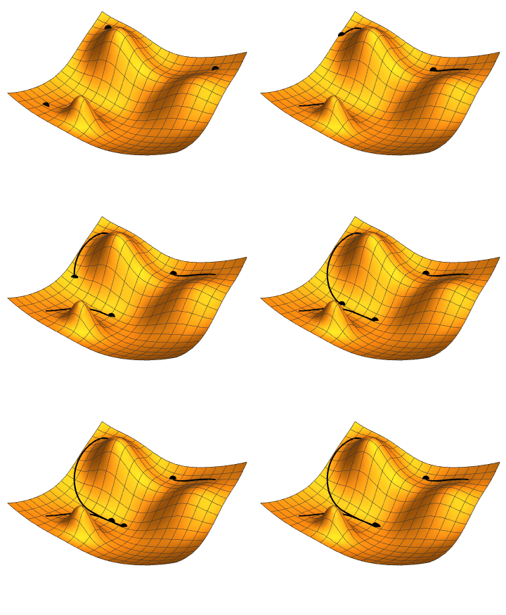
This works very well! In theory.

In practice, the landscape is rugged, as in the picture below

By following the gradient in such a landscape, variational optimization methods tend to get stuck in wrong regions of the parameter space, and provide false estimate.

PiecewiseInference.jl

PiecewiseInference.jl is a julia package that I have authored, which implements a method to smoothen the loss landscape, and that permits to automatically obtain the model parameter sensitivity. It is detailed in the following preprint

Boussange, V., Vilimelis-Aceituno, P., Pellissier, L., Mini-batching ecological data to improve ecosystem models with machine learning. bioRxiv (2022), 46 pages.

⚠️ We will shortly rename this preprint in a revised version, as the term “mini batching” is confusing. We now prefer the term “partitioning”

The method works by training the model on small chunks of data

Let’s use it to tune the paramters of our mechanitic model. We’ll group data points in groups of 11, indicated by the argument group_size = 11

using PiecewiseInference
include("utils.jl"); # some utility functions defining `inference_problem_args` and `piecewise_MLE_args`

loss_likelihood(data, pred, rg) = sum((log.(data) .- log.(pred)).^2)

infprob = InferenceProblem(model_mechanistic, 
                            p_mech; 
                            loss_likelihood, 
                            inference_problem_args...);

@time res_mech = piecewise_MLE(infprob;
                        group_size = 11,
                        data = data,
                        tsteps = tsteps,
                        optimizers = [Adam(1e-2)],
                        epochs = [500],
                        piecewise_MLE_args...)
piecewise_MLE with 101 points and 10 groups.
Current loss after 50 iterations: 14.972400665283203
Current loss after 100 iterations: 12.230918884277344
Current loss after 150 iterations: 11.497014045715332
Current loss after 200 iterations: 11.264657020568848
Current loss after 250 iterations: 11.19422721862793
Current loss after 300 iterations: 11.16870403289795
Current loss after 350 iterations: 11.156006813049316
Current loss after 400 iterations: 11.14731216430664
Current loss after 450 iterations: 11.141851425170898
Current loss after 500 iterations: 11.138410568237305
166.285066 seconds (1.17 G allocations: 177.010 GiB, 10.44% gc time, 27.02%
 compilation time: 0% of which was recompilation)
`InferenceResult` with model SimpleEcosystemModel

Now let’s plot what does this trained model predicts

simul_mech_forecast = simulate(model_mechanistic, 
                                p = res_mech.p_trained, 
                                u0 = data[:,1],
                                saveat = vcat(tsteps, tsteps_forecast), 
                                tspan = (0, tsteps_forecast[end]));

fig, ax = subplots(1, figsize=(7,4))
for i in 1:N
    ax.scatter(tsteps, 
                data[i,:], 
                label = labels_sp[i], 
                color = species_colors[i],
                s = 6.)
    ax.plot(tsteps[1:end], 
            simul_mech_forecast[i,1:length(tsteps)], 
            c = species_colors[i])
    ax.plot(tsteps_forecast, 
            simul_mech_forecast[i,length(tsteps)+1:end], 
            linestyle="--", 
            c = species_colors[i])
end
ax.set_ylabel("Species abundance")
ax.set_xlabel("Time (days)")
fig.set_facecolor("None")
ax.set_facecolor("None")
fig.legend()
display(fig)

Looks much better! The model now captures doubling period oscillations.

In summary, mechanistic models

  • ? Very good for extrapolating to novel scenarios
  • ? Hard to parametrise
  • ? Inacurate

Model selection

To improve the accuracy, one can try to formulate different models corresponding to alternative hypotheses about the processes driving the ecosystem dynamics. For instance, we could compare the performance of this model to an alternative model, which would capture some sort of dependence between the water availability and the resource growth rate.

If we find that the refined model performs better than the model with constant growth rate, we have learnt that water availability is an important driver that affects the ecosystem dynamics.

Hybrid models

Assume that we have no idea on what the dependence of the resource growth rate on water availability may look like.

To proceed, we can define a very generic parametric function that can capture any sort of dependence, and then try to learn the parameters of this function from the data.

Neural networks are parametric functions that are highly suited for this sort of task. So we’ll build a hyrbid model, which contains the mechanistic components of the previous model, but where the resource growth rate is parametrized by a neural network.

? + ?= ?

Below, we define the neural network, and the resource growth rate based on this neural net.

using Lux
rng = Random.default_rng()
# Multilayer FeedForward
hlsize = 5
neural_net = Lux.Chain(Lux.Dense(1,hlsize,rbf), 
                        Lux.Dense(hlsize,hlsize, rbf), 
                        Lux.Dense(hlsize,hlsize, rbf), 
                        Lux.Dense(hlsize, 1))
# Get the initial parameters and state variables of the model
p_nn, st = Lux.setup(rng, neural_net)
p_nn = p_nn |> ComponentArray

growth_rate_resource_nn(p_nn, water) = neural_net([water], p_nn, st)[1]

function hybrid_growth_rate(p, t)
    return [growth_rate_resource_nn(p.p_nn, water_availability(t)); p.r]
end
hybrid_growth_rate (generic function with 1 method)

Now we define our new hybrid model that implements this hybrid_growth_rate function

p_hybr = ComponentArray(H₂₁=p_mech.H₂₁,
                        H₃₂=p_mech.H₃₂,
                        q₂₁=p_mech.q₂₁,
                        q₃₂=p_mech.q₃₂,
                        r = p_mech.r[2:3],
                        K₁₁=p_mech.K₁₁,
                        A₁₁=p_mech.A₁₁,
                        p_nn = p_nn)

mp = ModelParams(;p=p_hybr,
                u0=u0_mech,
                solve_params...)

model_hybrid = SimpleEcosystemModel(; mp, 
                                    intinsic_growth_rate = hybrid_growth_rate,
                                    carrying_capacity,
                                    competition,
                                    resource_conversion_efficiency,
                                    feeding)
`Model` SimpleEcosystemModel

And we train it

infprob = InferenceProblem(model_hybrid, 
                            p_hybr; 
                            loss_likelihood, 
                            inference_problem_args...);

res_hybr = piecewise_MLE(infprob;
                    group_size = 11,
                    data = data,
                    tsteps = tsteps,
                    optimizers = [Adam(2e-2)],
                    epochs = [500],
                    piecewise_MLE_args...)
piecewise_MLE with 101 points and 10 groups.
Current loss after 50 iterations: 5.201906204223633
Current loss after 100 iterations: 3.6290767192840576
Current loss after 150 iterations: 3.519521713256836
Current loss after 200 iterations: 3.4955437183380127
Current loss after 250 iterations: 3.4787349700927734
Current loss after 300 iterations: 3.5343759059906006
Current loss after 350 iterations: 3.4698166847229004
Current loss after 400 iterations: 3.4563584327697754
Current loss after 450 iterations: 3.5980613231658936
Current loss after 500 iterations: 3.4506189823150635
`InferenceResult` with model SimpleEcosystemModel

The loss has signficiantly reduced. This means that this model better explains the dynamics, and as such, we have discovered that water avilability is indeed an important driver of ecosystem dynamics! Let’s plot the simulation output of this hyrbid model

simul_hybr_forecast = simulate(model_hybrid, 
                                p = res_hybr.p_trained, 
#                                 u0 = res_hybr.u0s_trained[1],
                                u0 = data[:,1],
                                saveat = vcat(tsteps, tsteps_forecast), 
                                tspan = (0, tsteps_forecast[end]));
fig, ax = subplots(1, figsize=(7,4))
for i in 1:N
    ax.scatter(tsteps, 
                data[i,:], 
                label = labels_sp[i], 
                color = species_colors[i],
                s = 6.)
    ax.plot(tsteps[1:end], 
        simul_hybr_forecast[i,1:length(tsteps)], 
            c = species_colors[i])
    ax.plot(tsteps_forecast, 
            simul_hybr_forecast[i,length(tsteps)+1:end], 
            linestyle="--", 
            c = species_colors[i])
end
ax.set_ylabel("Species abundance")
ax.set_xlabel("Time (days)")
fig.set_facecolor("None")
ax.set_facecolor("None")
fig.legend()
display(fig)

The cool thing is that although it contains a fully parametric component (the neural network), this hybrid can still extrapolate, because it is constrained by mechanistic processes.

plot_time_series(simulate(model_hybrid, 
                p = res_hybr.p_trained, 
                u0 = Float32[0., 0.060, 0.945], 
                saveat=0:dt:100.));

And what’s even cooler is that by interpreting the neural network, we can actually learn a new process: the shape of the dependence between the resource growth rate and the water availability!

water_avail = reshape(sort!(water_availability.(tsteps)),1,:)

p_nn_trained = res_hybr.p_trained.p_nn
gr = neural_net(water_avail, p_nn_trained, st)[1]


fig, ax = subplots(1)
ax.plot(water_avail[:], 
        gr[:], 
        label="Neural network",
        linestyle="--")

gr_true = model.mp.p[1] .* exp.(-0.5 .* water_avail.^2)
ax.plot(water_avail[:], gr_true[:], label="Ground truth")
ax.set_ylim(0,2)
ax.set_xlim(-2,2)
ax.legend()
xlabel("Water availability (normalized)")
ylabel("Resource basal growth rate")
display(fig)

Wrap-up

Hybrid approaches are the future! But they

  • Require
  • Requires differentiable programming and interoperability between scientific libraries
    • What
      is best at

    • But JAX is also very cool ?

Inverse ecosystem modeling made easy with PiecewiseInference.jl

By: julia | Victor Boussange

Re-posted from: https://vboussange.github.io/post/piecewiseinference/

Mechanistic ecosystem models permit to quantiatively describe how population, species or communities grow, interact and evolve. Yet calibrating them to fit real-world data is a daunting task. That’s why I’m excited to introduce PiecewiseInference.jl, a new Julia package that provides a user-friendly and efficient framework for inverse ecosystem modeling. In this blog post, I will guide you through the main features of PiecewiseInference.jl and provide a step-by-step tutorial on how to use it with a three-compartment ecosystem model. Whether you’re a quantitative ecologist or a curious data scientist, I hope this post will encourage you to join the effort and use and develop inverse ecosystem modelling methods to improve our understanding and predictions of ecosystems.

Preliminary steps

This tutorial relies on three packages that I have authored but are (yet) not registered on the official Julia registry. Those are

  • PiecewiseInference,
  • EcoEvoModelZoo: a package which provides access to a collection of ecosystem models,
  • ParametricModels: a wrapper package to manipulate dynamical models. Specifically, ParametricModels avoids the hassle of specifying, at each time you want to simulate an ODE model, boring details such as the algorithm to solve it, the time span, etc…

To easily install them on your machine, you’ll have to add my personal registry by doing the following:

using Pkg; Pkg.Registry.add(RegistrySpec(url = "https://github.com/vboussange/VBoussangeRegistry.git"))

Once this is done, let’s import those together with other necessary Julia packages for this tutorial.

using Graphs
using EcoEvoModelZoo
using ParametricModels
using LinearAlgebra
using UnPack
using OrdinaryDiffEq
using Statistics
using SparseArrays
using ComponentArrays
using PythonPlot

We use Graphs to create a directed graph to represent the food web to be considered The OrdinaryDiffEq package provides tools for solving ordinary differential equations, while the LinearAlgebra package is used for linear algebraic computations. The UnPack package provides a convenient way to extract fields from structures, and the ComponentArrays package is used to store and manipulate the model parameters conveniently. Finally, the PythonCall package is used to interface with Python’s Matplotlib library for visualization.

Definition of the forward model

Defining hyperparameters for the forward simulation of the model.

Next, we define the algorithm used for solving the ODE model. We also define the
absolute tolerance (abstol) and relative tolerance (reltol) for the solver.
tspan is a tuple representing the time range we will simulate the system for,
and tsteps is a vector representing the times we want to output the simulated
data.

alg = BS3()
abstol = 1e-6
reltol = 1e-6
tspan = (0.0, 600)
tsteps = range(300, tspan[end], length=100)
300.0:3.0303030303030303:600.0

Defining the foodweb structure

We’ll define a 3-compartment ecosystem as presented in McCann et al. (1994). We will use SimpleEcosystemModel from EcoEvoModeZoo.jl, which requires as input a foodweb structure. Let’s use a DiGraph to represent it.

N = 3 # number of compartment

foodweb = DiGraph(N)
add_edge!(foodweb, 2 => 1) # C to R
add_edge!(foodweb, 3 => 2) # P to C
true

The N variable specifies the number of
compartments in the model. The add_edge! function is used to add edges to the
graph, specifying the flow of resources between compartments.

For fun, let’s just plot the foodweb. Here we use the PythonCall and PythonPlot
packages to visualize the food web as a directed graph using networkx and numpy.
We create a color list for the different species, and then create a directed
graph g_nx with networkx using the adjacency matrix of the food web. We also
specify the position of each node in the graph, and use nx.draw to draw the
graph with

using PythonCall
nx = pyimport("networkx")
np = pyimport("numpy")
species_colors = ["tab:red", "tab:green", "tab:blue"]

g_nx = nx.DiGraph(np.array(adjacency_matrix(foodweb)))
pos = Dict(0 => [0, 0], 1 => [0.2, 1], 2 => [0, 2])
labs = Dict(0 => "Resource", 1 => "Consumer", 2 => "Prey")

fig, ax = subplots(1)
nx.draw(g_nx, pos, ax=ax, node_color=species_colors, node_size=1000, labels=labs)
display(fig)

Defining the ecosystem model

Now that we have defined the foodweb structure, we can build the ecosystem
model, which will be a SimpleEcosystemModel from EcoEvoModelZoo.

The next several functions are required by SimpleEcosystemModel and define the
specific dynamics of the model. The intinsic_growth_rate function specifies
the intrinsic growth rate of each compartment, while the carrying_capacity
function specifies the carrying capacity of each compartment. The competition
function specifies the competition between and within compartments, while the
resource_conversion_efficiency function specifies the efficiency with which
resources are converted into consumer biomass. The feeding function specifies
the feeding interactions between compartments.

intinsic_growth_rate(p, t) = p.r

function carrying_capacity(p, t)
    @unpack K₁₁ = p
    K = vcat(K₁₁, ones(N - 1))
    return K
end

function competition(u, p, t)
    @unpack A₁₁ = p
    A = spdiagm(vcat(A₁₁, 0, 0))
    return A * u
end

resource_conversion_efficiency(p, t) = ones(N)
resource_conversion_efficiency (generic function with 1 method)

To define the feeding processes, we use adjacency_matrix to get the adjacency matrix of the food web. We then use findnz from SparseArrays to get the row and column indices of the non-zero entries in the adjacency matrix, which we store in I and J. Those are then used to generate sparse matrices required for defining the functional responses of each species considered. The sparse matrices’ non-zero coefficients are the model parameters to be fitted.

using SparseArrays
W = adjacency_matrix(foodweb)
I, J, _ = findnz(W)
([2, 3], [1, 2], [1, 1])
function feeding(u, p, t)
    @unpack H₂₁, H₃₂, q₂₁, q₃₂ = p

    # handling time
    H = sparse(I, J, vcat(H₂₁, H₃₂), N, N)

    # attack rates
    q = sparse(I, J, vcat(q₂₁, q₃₂), N, N)

    return q .* W ./ (one(eltype(u)) .+ q .* H .* (W * u))
end
feeding (generic function with 1 method)

We are done defining the ecological processes.

Defining the ecosystem model parameters for generating a dataset

The parameters for the ecosystem model are defined using a ComponentArray. The
u0_true variable specifies the initial conditions for the simulation. The
ModelParams type from the ParametricModels package is used to specify the
model parameters and simulation settings. Finally, the SimpleEcosystemModel
type from the EcoEvoModelZoo package is used to define the ecosystem model.

p_true = ComponentArray(H₂₁=[1.24],
                        H₃₂=[2.5],
                        q₂₁=[4.98],
                        q₃₂=[0.8],
                        r=[1.0, -0.4, -0.08],
                        K₁₁=[1.0],
                        A₁₁=[1.0])

u0_true = [0.77, 0.060, 0.945]

mp = ModelParams(; p=p_true,
    tspan,
    u0=u0_true,
    alg,
    reltol,
    abstol,
    saveat=tsteps,
    verbose=false, # suppresses warnings for maxiters
    maxiters=50_000
)
model = SimpleEcosystemModel(; mp, intinsic_growth_rate,
    carrying_capacity,
    competition,
    resource_conversion_efficiency,
    feeding)
`Model` SimpleEcosystemModel

Let’s run the model to generate a dataset! There is nothing more simple than that. Let’s also plot it,
to get a sense of what it looks like.

data = simulate(model, u0=u0_true) |> Array

# plotting
using PythonPlot;
function plot_time_series(data)
    fig, ax = subplots()
    for i in 1:N
        ax.plot(data[i, :], label="Species $i", color = species_colors[i])
    end
    # ax.set_yscale("log")
    ax.set_ylabel("Species abundance")
    ax.set_xlabel("Time (days)")
    fig.set_facecolor("None")
    ax.set_facecolor("None")
    fig.legend()
    return fig
end

display(plot_time_series(data))

Let’s add a bit of noise to the data to simulate experimental errors. We proceed by adding
log normally distributed noise, so that abundance are always positive (negative abundance would not make sense, but could happen when adding normally distributed noise!).

data = data .* exp.(0.1 * randn(size(data)))

display(plot_time_series(data))

Inversion with PiecewiseInference.jl

Now that we have set up our model and generated some data, we can proceed with the inverse modelling using PiecewiseInference.jl.

PiecewiseInference.jl allows to perform inversion based on a segmentation method that partitions the data into short time series (segments), each treated independently and matched against simulations of the model considered. The segmentation approach helps to avoid the ill-behaved loss functions that arise from the strong nonlinearities of ecosystem models, when formulation the inference problem. Note that during the inversion, not only the parameters are inferred, but also the initial conditions, which are necessary to simulate the ODE model.

Definition of the InferenceProblem

We first import the packages required for the inversion. PiecewiseInference is the
main package used, but we also need OptimizationFlux for the Adam optimizer,
and SciMLSensitivity to define the sensitivity method used to differentiate
the forward model.

using PiecewiseInference
using OptimizationFlux
using SciMLSensitivity

To initialize the inversion, we set the initial values for the parameters in p_init to those of p_true but modify the H₂₁ parameter.

p_init = p_true
p_init.H₂₁ .= 2.0 #
1-element view(::Vector{Float64}, 1:1) with eltype Float64:
 2.0

Next, we define a loss function loss_likelihood that compares the observed data
with the predicted data. Here, we use a simple mean-squared error loss function while log transforming the abundance, since the noise is log-normally distributed.

loss_likelihood(data, pred, rg) = sum((log.(data) .- log.(pred)) .^ 2)# loss_fn_lognormal_distrib(data, pred, noise_distrib)
loss_likelihood (generic function with 1 method)

We then define the InferenceProblem, which contains the forward
model, the initial parameter values, and the loss function.

infprob = InferenceProblem(model, p_init; loss_likelihood);

It is also handy to use a callback function, that will be called after each iteration of the optimization routine, for visualizing the progress of the inference. Here, we use it to track the loss value and plot the data against the model predictions.

info_per_its = 50
include("cb.jl") # defines the `plotting_fit` function
function callback(p_trained, losses, pred, ranges)
    if length(losses) % info_per_its == 0
        plotting_fit(losses, pred, ranges, data, tsteps)
    end
end
callback (generic function with 1 method)

piecewise_MLE hyperparameters

To use piecewise_MLE, the main function of PiecewiseInference to estimate the parameters that fit the observed data, we need to decide on two critical hyperparameters

  • group_size: the number of data points that define an interval, or segment. This number is usually small, but should be decided upon the dynamics of the model: to more nonlinear is the model, the lower group_size should be. We set it here to 11
  • batch_size: the number of intervals, or segments, to consider on a single epoch. The higher the batch_size, the more computationally expensive a single iteration of piecewise_MLE, but the faster the convergence. Here, we set it to 5, but could increase it to 10, which is the total number of segments that we have.

Another critical parameter to be decided upon is the automatic differentiation backend used to differentiate the ODE model. Two are supported, Optimization.AutoForwardDiff() and Optimization.Autozygote(). Simply put, Optimization.AutoForwardDiff() is used for forward mode sensitivity analysis, while Optimization.Autozygote() is used for backward mode sensitivity analysis. For more information on those, please refer to the documentation of Optimization.jl.

Other parameters required by piecewise_MLE are

  • optimizers specifies the optimization algorithm to be used for each batch. We use the Adam optimizer, which is the go-to optimizer to train deep learning models. It has a learning rate parameter that controls the step size at each iteration. We have chosen a value of 1e-2 because it provides good convergence without causing numerical instability,

  • epochs specifies the number of epochs to be used for each batch. We chose a value of 500 because it is sufficient to achieve good convergence,

  • info_per_its specifies after how many iterations the callback function should be called

  • verbose_loss prints the value of the loss function during training,

@time res = piecewise_MLE(infprob;
                        adtype = Optimization.AutoZygote(),
                        group_size = 11,
                        batchsizes = [5],
                        data = data,
                        tsteps = tsteps,
                        optimizers = [Adam(1e-2)],
                        epochs = [500],
                        verbose_loss = true,
                        info_per_its = info_per_its,
                        multi_threading = false,
                        cb = callback)
piecewise_MLE with 100 points and 10 groups.
Current loss after 50 iterations: 36.745952018526495
Current loss after 100 iterations: 15.064711239454626
Current loss after 150 iterations: 9.993029255013324
Current loss after 200 iterations: 7.994491307947515
Current loss after 250 iterations: 6.500818892986831
Current loss after 300 iterations: 5.3892647156988565
Current loss after 350 iterations: 3.0351181646280514
Current loss after 400 iterations: 2.674445730720996
Current loss after 450 iterations: 3.1591980829795676
Current loss after 500 iterations: 2.4343376293865995
157.765049 seconds (1.70 G allocations: 154.827 GiB, 10.16% gc time, 31.31%
 compilation time: 1% of which was recompilation)
`InferenceResult` with model SimpleEcosystemModel

Finally, we can examine the results of the inversion. We can look at the final parameters, and the initial conditions inferred for each segement:

# Some more code
p_trained = res.p_trained
u0s_trained = res.u0s_trained

function print_param_values(p_trained, p_true)
    for k in keys(p_trained)
        println(string(k))
        println("trained value = "); display(p_trained[k])
        println("true value ="); display(p_true[k])
    end
end

print_param_values(p_trained, p_true)
H₂₁
trained value = 
1-element Vector{Float64}:
 1.4786844814887716
true value =
1-element Vector{Float64}:
 2.0
H₃₂
trained value = 
1-element Vector{Float64}:
 1.891238277791975
true value =
1-element Vector{Float64}:
 2.5
q₂₁
trained value = 
1-element Vector{Float64}:
 4.550896291686214
true value =
1-element Vector{Float64}:
 4.98
q₃₂
trained value = 
1-element Vector{Float64}:
 0.7250599871665505
true value =
1-element Vector{Float64}:
 0.8
r
trained value = 
3-element Vector{Float64}:
  0.8705446490535288
 -0.30124597815843823
 -0.08241879418666838
true value =
3-element Vector{Float64}:
  1.0
 -0.4
 -0.08
K₁₁
trained value = 
1-element Vector{Float64}:
 1.0397189294700315
true value =
1-element Vector{Float64}:
 1.0
A₁₁
trained value = 
1-element Vector{Float64}:
 0.972947353012839
true value =
1-element Vector{Float64}:
 1.0

Your turn to play!

You can try to change e.g. the batch_sizes and the group_size. How do those parameters influence the quality of the inversion?

Conclusion

PiecewiseInference.jl provides an efficient and flexible way to perform inference on complex ecological models, making use of automatic differentiation and optimizers traditionally used in Machine Learning. The segmentation method implemented in PiecewiseInference.jl regularizes the inference problem and enables inverse modelling of complex dynamical systems, for which standard methods would otherwise fail.

Furthermore, PiecewiseInference.jl together with EcoEvoModelZoo.jl offer a powerful toolkit for ecologists and evolutionary biologists to benchmark and validate models against data. The combination of theoretical modelling and data can provide new insights into complex ecological systems, helping us to better understand and predict the dynamics of biodiversity.

We invite users to explore these packages and contribute to their development, by adding new models to the EcoEvoModelZoo.jl and improve the features of PiecewiseInference.jl. With these tools, we can continue to push the boundaries of ecological modelling and make important strides towards a more sustainable future.

Appendix

You can find the corresponding tutorial as a .jmd file at https://github.com/vboussange/MyTutorials.
Please contact me, if you have found a mistake, or if you have any comment or suggestion on how to improve this tutorial.

A practical introduction to approximate Bayesian computation

By: julia | Victor Boussange

Re-posted from: https://vboussange.github.io/post/abc_inference/

Introduction

In this tutorial, we’ll learn the basics of approximate Bayesian computation (ABC).
ABC is a very flexible inference method that is quite intuitive, and that you can apply to almost any model type. As such, it is quite handy to have it in one’s toolbox! To build up an intuition of the method, we’ll perform ABC on a very simple ecosystem model, using Julia, and will visualize graphically the inference results.

Package loading

We first need to load a few packages.

cd(@__DIR__)
using Pkg; Pkg.activate(".")
using Random
using LinearAlgebra
import Optimisers:destructure # required to simplify parameter indexing
using UnPack # for parameter indexing
using ApproxBayes # ABC toolbox
using Distributions # useful to define the priors
using OrdinaryDiffEq # ODE solver library
using ParametricModels # convenience package for ODE models. /!\ package not registered

It is always important to make your work reproducible, so we’ll set manually a seed to the random number generator.

# Set a seed for reproducibility.
Random.seed!(11);

Model definition and data generation

What we’ll do is to implement an Ordinary Differential Equation model, which will be used to generate synthetic data and further perform the inference. The idea here is to consider this synthetic data as our empirical data, and pretend that we do not know which parameters generated this data. Our goal is then to recover the generating parameters.

We’ll consider a predator-prey ecological model, the Lotka-Volterra equations. This model has a total of four different parameters $\alpha, \beta, \gamma, \delta$, that describe the interactions between the two species. For the sake of simplicity, we’ll assume that we know perfectly the parameters $\gamma, \delta$, and seek to infer $\alpha$ and $\beta$. Assuming to know $\gamma, \delta$ is of course a very unrealistic assumption… but a handy assumption to develop an intuition about parameter inference.

We use ParametricModels.jl to define our model. ParametricModels.jl is a simple wrapper around OrdinaryDiffEq.jl, that allows to play around with the model without bothering further about the details of the numerical solve. This makes it easier to simulate repeatedly an ODE model. For readability and maintenance, we’ll encapsulate the parameters in a NamedTuple.

# Declaration of the model
ParametricModels.@model LotkaVolterra
# Definition of the model
function (lv::LotkaVolterra)(du, u, p, t)
    # Model parameters
    @unpack α, β, = p
    # Current state
    x, y = u
    # fixed parameters
    γ = 3.0
    δ = 1.0

    # Evaluate differential equations
    du[1] = (α[] - β[] * y) * x # prey
    du[2] = (δ * x - γ) * y # predator

    return nothing
end
# Define initial-value problem.
u0 = [1.0, 1.0]
p = (α=[1.5], β=[1.0])
tspan = (0.0, 10.0)

model = LotkaVolterra(ModelParams(;u0, p, tspan, alg=Tsit5(), saveat=0.1))
sol = simulate(model);

And here we go, we have our model defined!

As an exercise, you could try to write the same model with OrdinaryDiffEq.jl.

Let’s now plot the model output.
We first need to import some plotting utilities.
For plotting, I tend to use PyPlot.jl, which is a wrapper around the Python library matplotlib. I find it much more convenient than the Julia package Plots.jl, in the sense that it contains more utility functions. It is always a good idea to load in parallel PyCall.jl, which allows to import other utility funtions from Python.

using PyPlot # to plot 3d landscape
using PyCall

Here is a plot of the model output without noise:

fig = PyPlot.figure()
PyPlot.plot(sol')
display(fig)

We now use sol to generate synthetic data containing some noise (in mathematical terms, we call this a Gaussian white noise, which follows $\mathcal{N}(0,\sigma)$ where $\sigma = 0.8$.

σ = 0.8
odedata = Array(sol) + σ * randn(size(Array(sol)))
fig = figure()
PyPlot.plot(odedata')
display(fig)

The model and the synthetic data are ready, let’s get started with ABC!

Approximate Bayesian computation

For ABC, one needs to define a function $\rho$ that measures the distance between the model output $\hat \mu$ (in the picture below, $\mu_i$) and the empirical data $\mu$.

source: Wikipedia

In our case, the empirical data available (odedata) allows us to explicitly define the likelihood of the model given the data. As a distance function, we therefore can first use the negative log of the likelihood. For additive Gaussian noise, the likelihood of the model is given by

$$\begin{split}
p(y_{1:K} | \theta, \mathcal{M}) &= \prod_{i=1}^K p(y_{i} | \theta, \mathcal{M})\\
&= \prod_{k=1}^K \frac{1}{\sqrt{(2\pi)^d|\Sigma_y|}} \exp \left(-\frac{1}{2} \epsilon_k^{T} \Sigma_y^{-1} \epsilon_k \right)
\end{split}$$

where $\epsilon_k \equiv \epsilon(t_k) = y(t_k) – h\left(\mathcal{M}(t_k, \theta)\right)$ and $\Sigma_y = \sigma^2 I$ in our case.

So let’s translate all this in Julia code.

ApproxBayes.jl requires as input a function simfunc(params, constants, data), which plays the role of the $\rho$ function. It should return the distance value, as well as a second value that may be used for logging. To make things simple, we’ll return nothing for this second value.

Because ApproxBayes.jl requires that params is an array (params <: AbstractArray), we further use a special trick relying on the function Optimiser.destructure. This utility function allows to generate a function re that can recover a NamedTuple from a vector. Very useful in combination with the utility macro @unpack!

_, re = destructure(p)
function log_likelihood(p; odedata=odedata)
    p_tuple = re(p)
    pred = simulate(model, p=p_tuple)
    return sum([loglikelihood(MvNormal(zeros(2), LinearAlgebra.I * σ^2), odedata[:,i] - pred[:,i]) for i in 1:size(odedata,2)])
end
function simfunc(params, constants, data)
    ρ = - log_likelihood(params, odedata=data)
    return ρ, nothing
end

# testing function
simfunc([1.0, 1.2], nothing, odedata)
(1403.0830673958446, nothing)

Now that the distance function is implemented, we define the priors on the parameters $\alpha, \beta$

priors = [truncated(Normal(1.1, 1.), 0.5, 2.5), # for α and β
            truncated(Normal(1.1, 1.), 0., 2.)]
num_samples = 500
max_iterations = 1e5
ϵ = 2.0
abcsetup = ABCRejection(simfunc,
                        length(priors),
                        ϵ,
                        ApproxBayes.Prior(priors);
                        nparticles=num_samples,
                        maxiterations=max_iterations)

abcresult = runabc(abcsetup, odedata, progress=true, parallel=true)
Preparing to run in parallel on 5 processors
Number of simulations: 1.00e+05
Acceptance ratio: 5.00e-03

Median (95% intervals):
Parameter 1: 1.51 (1.48,1.53)
Parameter 2: 1.00 (0.86,1.16)

And here we go: abcresult informs us that the ABC inference could indeed recover the parameters that generated the data!

Visualizing the inference process

To better understand what has happened, let’s plot the parameters that have been accepted by the sampler, together with the real likelihood landscape. As a first step, let’s visualise the real likelihoood landscape.


αs = range(1.45, 1.55, length=100)
βs = range(0.8, 1.3, length=100)
likelihoods = Float64[]
for α in αs
    for β in βs
        p = [α, β]
        push!(likelihoods, log_likelihood(p))
    end
end

likelihoods = exp.(likelihoods); # exponentiating, to make it visually nicer

We now define an Axes3D, as you would do it in Python:

# Plotting 3d landscape
fig = plt.figure()
ax = Axes3D(fig, computed_zorder=false);

We’ll import numpy into Julia, to easily construct the meshgrid required by the matplotlib function plot_surface.

np = pyimport("numpy") # used for plotting
X, Y = np.meshgrid(αs, βs)


# fig.savefig("perturbed_p.png", dpi = 300, bbox_inches="tight")
ax.plot_surface(X .|> Float64,
    Y .|> Float64,
    reshape(likelihoods, (length(αs), length(βs))) .|> Float64,
    edgecolor="0.7",
    linewidth=0.2,
    cmap="Blues", zorder=-1)
ax.set_xlabel(L"p_1")
ax.set_ylabel(L"p_2")
ax.set_zlabel("Likelihood", x=2)
ax.set_xticks([])
ax.set_yticks([])
ax.set_zticks([])

# make the panes transparent
ax.xaxis.set_pane_color((1.0, 1.0, 1.0, 0.0))
ax.yaxis.set_pane_color((1.0, 1.0, 1.0, 0.0))
ax.zaxis.set_pane_color((1.0, 1.0, 1.0, 0.0))
# make the grid lines transparent
ax.xaxis._axinfo["grid"]["color"] = (1.0, 1.0, 1.0, 0.0)
ax.yaxis._axinfo["grid"]["color"] = (1, 1, 1, 0)
ax.zaxis._axinfo["grid"]["color"] = (1, 1, 1, 0)

fig.tight_layout()
fig.set_facecolor("None")
ax.set_facecolor("None")

for p in eachrow(abcresult.parameters)
    ax.scatter(p[1], p[2], exp.(log_likelihood(p)), c="tab:red", zorder=100, s = 0.5)
end
p = abcresult.parameters[1,:]
ax.scatter(p[1], p[2], exp(log_likelihood(p)), c="tab:red", zorder=100, s = 2., label="Accepted simulation")
ax.legend()
display(fig)

Cool, right?

Summary statistics

It may be useful, or necessary, to use summary statistics of the data instead of the full likelihood, to be provided to the distance function. Summary statistics are values calculated from the data to represent the maximum amount of information in the simplest possible form. Using summary statistics allows to reduce the dimensionality of the data, which increases the probability of accepting the model output. In our case, the dimensionality correponds to the number of time steps multiplied by the number of state variables). Using summary statistics may prove useful to improve the convergence of the inference process, were the inference not converge using the likelihood function. But because it reduces the amount of information provided to the inference method, it may also hamper a precise characterisation of the model parameter values.

Mean and variance

As summary statistics, we can here compute the mean and covariance matrix of the state variables, and use those to define the distance between the model output and the data.

compute_summary_stats(data) = [mean(data,dims=2); cov(data, dims=2)[:]]
ss_data = compute_summary_stats(odedata)
6×1 Matrix{Float64}:
 2.966416873264894
 1.5414956648089986
 4.784360022666909
 0.07385819785251807
 0.07385819785251807
 2.680060599643699

Let’s now proceed similarly to above

function simfunc(params, constants, ss_data)
    p_tuple = re(params)
    pred = simulate(model, p=p_tuple)
    ss_pred = compute_summary_stats(pred)
    ρ = sum((ss_pred .- ss_data).^2) # taking euclidean distance between
    return ρ, nothing
end

simfunc([1.0, 1.2], nothing, ss_data)

priors = [truncated(Normal(1.1, 1.), 0.5, 2.5), # for α and β
            truncated(Normal(1.1, 1.), 0., 2.)]
num_samples = 500
max_iterations = 1e5
ϵ = 0.15
abcsetup = ABCRejection(simfunc,
                        length(priors),
                        ϵ,
                        ApproxBayes.Prior(priors);
                        nparticles=num_samples,
                        maxiterations=max_iterations)

abcresult = runabc(abcsetup, ss_data, progress=true, parallel=true)
Preparing to run in parallel on 5 processors
Number of simulations: 1.00e+05
Acceptance ratio: 5.00e-03

Median (95% intervals):
Parameter 1: 2.10 (1.98,2.30)
Parameter 2: 1.11 (1.01,1.23)

As you can see, the results of the inference or much less accurate.

Which other summary statistics of the time series could you think of? You can find below tests with other summary statistics.

And that’s it for today! Hopefully this tutorial has given you some basics and intuition on ABC, and how to use in Julia.

Further references

Appendix

You can find the corresponding tutorial as a .jmd file at https://github.com/vboussange/MyTutorials. To use ParametricModels.jl, follow the procedure indicated on the github repo.
Please contact me, if you have found a mistake, or if you have any comment or suggestion on how to improve this tutorial.

Summary statistics with Fourier transforms

using FFTW
# Fourier Transform of the data
F = fft(odedata .- mean(odedata,dims=2)) |> fftshift
# freqs = fftfreq(size(odedata, 2), 1.0/Ts) |> fftshift
fig = figure()
plot(1:size(odedata,2), abs.(F)')
display(fig)

Let’s select the frequency which frequency is predominent, and consider it for our summary statistics

freq_x = sortperm(abs.(F[1,:]))[end-1:end] # selecting the two most important frequencies
freq_y = sortperm(abs.(F[1,:]))[end-1:end] # selecting the two most important frequencies
@assert freq_x == freq_y # both prey and predator data peak at the same frequencies

function compute_summary_stats(data)
    F = fft(Array(data)) |> fftshift
    return abs.(F[:,freq_x])
end
ss_data = compute_summary_stats(Array(odedata))
simfunc([1.0, 1.2], nothing, ss_data)
(29583.477061802652, nothing)

Let’s now proceed similarly to above

priors = [truncated(Normal(1.1, 1.), 0.5, 2.5), # for α and β
            truncated(Normal(1.1, 1.), 0., 2.)]
num_samples = 500
max_iterations = 1e5
ϵ = 0.15
abcsetup = ABCRejection(simfunc,
                        length(priors),
                        ϵ,
                        ApproxBayes.Prior(priors);
                        nparticles=num_samples,
                        maxiterations=max_iterations)

abcresult = runabc(abcsetup, ss_data, progress=true, parallel=true)
Preparing to run in parallel on 5 processors
Number of simulations: 1.00e+05
Acceptance ratio: 5.00e-03

Median (95% intervals):
Parameter 1: 1.44 (1.05,2.38)
Parameter 2: 0.92 (0.26,0.99)

Although we have quite a large uncertainty on the parameters, the Fourier transform-based summary statistics seem to contain more relevant information, and this is reflected on the more accurate value of the inferred parameters.

Summary statistics with auto-correlation

Here we use the autocorrelation function to build our summary statistics. The default lag value of the autocor in Julia reduces the dimension of the data to a matrix of size 21x2.

using StatsBase
autocor_ss = autocor(odedata') 
fig = figure()
plot(1:size(autocor_ss,1), autocor_ss)
display(fig)

If we were to compute the lag from $t = 0$ to $t = t_{\text{max}}$, we would obtain a sinusoidal curve, similar to the time series raw data.

compute_summary_stats(data) = autocor(Array(data)')
ss_data = compute_summary_stats(odedata)
simfunc([1.0, 1.2], nothing, ss_data)
(1.4530748281677037, nothing)

Let’s now proceed similarly to above

priors = [truncated(Normal(1.1, 1.), 0.5, 2.5), # for α and β
            truncated(Normal(1.1, 1.), 0., 2.)]
num_samples = 500
max_iterations = 1e5
ϵ = 0.15
abcsetup = ABCRejection(simfunc,
                        length(priors),
                        ϵ,
                        ApproxBayes.Prior(priors);
                        nparticles=num_samples,
                        maxiterations=max_iterations)

abcresult = runabc(abcsetup, ss_data, progress=true, parallel=true)
Preparing to run in parallel on 5 processors
Number of simulations: 1.00e+05
Acceptance ratio: 5.00e-03

Median (95% intervals):
Parameter 1: 1.53 (1.45,1.61)
Parameter 2: 0.35 (0.29,0.41)