Author Archives: Jacob Quinn

Generated constant propagation; hold on to your britches!

By: Jacob Quinn

Re-posted from: https://quinnj.home.blog/2019/06/20/generated-constant-propagation-hold-on-to-your-britches/

In a recent JuliaLang Discourse post, OP was looking for a simple way to convert their Vector{CustomType} to a DataFrame, treating each CustomType element as a “row”, with the fields of CustomType as fields in the row. The post piqued my interest, given my work on the Tables.jl interface over the last year. Tables.jl is geared specifically towards creating generic access patterns to “table” like sources, specifically providing Tables.rows and Tables.columns as two ways to access table data from any source. Tables.columns returns a “property-accessible object” of iterators, while Tables.rows returns the dual: an iterator of “property-accessible objects” (property-accessible object here is defined as any object that supports both propertynames(obj) and getproperty(obj, prop), which includes all custom structs by default).

I decided to respond by showing how simple it can be to “hook in” to the Tables.jl world of interop; my code looked like:

using DataFrames, Random, Tables

struct Mine
a::Int
b::Float64
c::Matrix{Float64}
end

Tables.istable(::Type{Vector{Mine}}) = true
Tables.rowaccess(::Type{Vector{Mine}}) = true
Tables.rows(x::Vector{Mine}) = x
Tables.schema(x::Vector{Mine}) = Tables.Schema((:a, :b), Tuple{Int, Float64})

Random.seed!(999)
v = [Mine(rand(1:10), rand(), rand(2,2)) for i ∈ 1:10^6];
df = DataFrame(v)

But when doing a quick benchmark of the conversion from Vector{Mine} to DataFrame, it was 3x-5x slower than other methods already proposed. Huh? I started digging. One thing I noticed was by ***not*** defining Tables.schema, the code was a bit faster! That led me to assume something was up in our schema-based row-to-column code.

Part of the challenge with this functionality is wrestling with providing a fast, type-stable method for building up strongly-typed columns for a set of rows with arbitrary number of columns and types. Just iterating over a row in a for-loop, accessing each field programmatically can be disastrous; because each extracted field value in the hot for-loop could be a number of types, the compiler can’t do much more than create a Core.Box to put arbitrary values in, then pull out again for inserting into the vector we’re building up. Yuck, yuck, yuck; if you see Core.Boxs in your @code_typed output, or values inferred as Any, it’s an indication the compiler just couldn’t figure out anything more specific, and in a hot for-loop called over and over and over again, any hope of performance is toast.

Enter meta-programming: Tables.jl tries to judiciously employ the use of @generated functions to help deal w/ the issue here. Specifically, when doing this rows-to-columns conversion, with a known schema, Tables.eachcolumn can take the column names/types as input, and generate a custom function with this aforementioned “hot for-loop” unrolled. That is, instead of:

for rownumber = 1:number_of_rows
row = rows[rownumber]
for i = 1:ncols
column[i][rownumber] = getfield(row, i)
end

end

For a specific table input’s schema, the generated code looks like:

for rownumber = 1:number_of_rows
row = rows[rownumber]
column[1][rownumber] = getfield(row, 1)
column[2][rownumber] = getfield(row, 2)
# etc.
end

What makes this code ***really*** powerful is the compiler’s ability to do “constant propagation”, which means that, while compiling, when it encounters getfield(row, 1), it can realize, “hey, I know that row is a Mine type, and I see that they’re calling getfield to get the 1 field, and I happen to know that the 1 field of Mine is an Int64, so I’ll throw that information into dataflow analysis so things can get further inlined/optimized”. It’s really the difference between the scenario I described before of the compiler just having to treat the naive for-loop values as Any vs. recognizing that it can figure out the exact types to expect which can make the operation we’re talking about here boil down to a very simple “load”, then “store”, without needing to box/unbox or rely on runtime dynamic dispatch based on types.

Back to the original issue: why was this code slower than the unknown schema case? Well, it turns out that our generated code was actually trying to be clever by calculating a run-length encoding of consecutive types for a schema, then generating mini type-stable for-loops; i.e. the generated code looked like:

for rownumber = 1:number_of_rows
row = rows[rownumber]
# if columns 1 & 2 are Int64
for col = 1:2
column[col][rownumber] = getfield(row, col)
end
# column 3 is a Float64
for col = 3:3
column[col][rownumber] = getfield(row, col)
end
# columns 4 & 5 are Int64 again
for col = 4:5
column[col][rownumber] = getfield(row, col)
end
# etc.
end

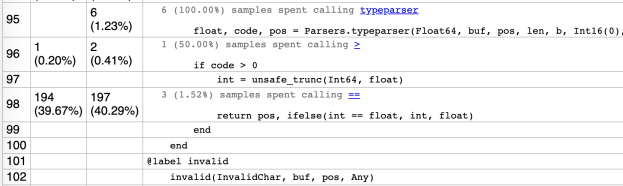
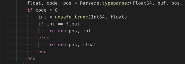
While this is clever, and can generate less code when schema types tend to be “sticky” (i.e. lots of the same type consecutively), the problem is in the getfield(row, col) call. Even though the call to each getfield ***should*** be type-stable, as calculated from our run-length encoding, the compiler unfortunately can’t figure that out inside these mini type-stable for-loops. This means no super-inlining/optimizations, so things end up being slower.

So what’s the conclusion here? What can be done? The answer was pretty simple, instead of trying to be extra clever with run-length encodings, if the schema is small enough, just generate the getfield calls directly for each column. The current heuristic is for schemas with less than 100 columns, the code will be generated directly, and for larger schema cases, we’ll try the run-length encoding approach (since it’s still more efficient than the initial naive approach).

Hope you enjoyed a little dive under the hood of Tables.jl and some of the challenges the data ecosystem faces in the powerful type system of Julia. Ping me on twitter with any thoughts or questions.

Cheers.

Tricksy Tuple Types…

By: Jacob Quinn

Re-posted from: https://quinnj.home.blog/2019/06/19/tricksy-tuple-types/

Some of you may be aware of my obsession with JSON libraries, and it’s true, there’s something about simple data formats that sends my brain into endless brainstorming of ways to optimize reading, writing, and object-mapping in the Julia language. JSON3.jl is my latest attempt at a couple of new ideas for JSON <=> Julia fun. The package is almost ready for a public release, and I promise I’ll talk through some of the fun ideas going on there, but today, just wanted to point out a tricky performance issue that took a bit of sleuthing to track down.

Here’s the scenario: we have a string of JSON like {"a": 1}, super simple right? In the standard Julia JSON.jl library, you just call JSON.parse(str) and get back a Dict{String, Any}. In JSON3.jl, we have a similar “plain parse” option which looks like JSON3.read(str), which returns a custom JSON3.Object type which I can talk about in another post in more detail. Another option in JSON3.jl, is to do JSON3.read(str, Dict{String, Any}), i.e. we can specify the type we’d like to parse from any string of JSON. While doing some quick benchmarking to make sure things look reasonable, I noticed JSON3.jl was about 2x slower compared to both JSON.parse, and JSON3.read(str, Dict{String, Int}). Hmmm, what’s going on here??

I first turned to profiling, and used the wonderful StatProfilerHTML.jl package to inspect my profiling results. That’s when I noticed around ~40% of the time was spent on a seemingly simple line of code:

Hmmmm……a return statement with a simple ifelse call? Seems fishy. Luckily, there’s a fun little project called Cthulhu.jl, which allows debugger “stepping” functionality with Julia’s unparalleled code inspection tools (@code_lowered, @code_typed, @code_llvm, etc.). As I “descended into madness” to take a look at the @code_typed of this line of code, I found this:

%1865 = (JSON3.ifelse)(%1864, %1857, %1851)::Union{Float64, Int64}
%1866 = (Core.tuple)(%1853, %1865)::Tuple{Int64,Union{Float64, Int64}}

Ruh-roh Shaggy…….the issue here is this Tuple{Int64,Union{Float64,Int64}} return type. It’s not concrete and leads to worse type inference in later code that tries to access this tuple’s second element. This is also undesirable because we know that the value should be either an Int64 or Float64, so ideally we could structure things so that code generation can just do a single branch and generate nice clean code the rest of the way down. If we change the code to:

Let’s take another cthulic descent and check out the generated code:

%1863 = (%1857 === %1862)::Bool
│ │ @ float.jl:484 within `==' @ float.jl:482
│ │┌ @ bool.jl:40 within `&'
│ ││ %1864 = (Base.and_int)(%1861, %1863)::Bool
│ └└
└──── goto #691 if not %1864
@ /Users/jacobquinn/.julia/dev/JSON3/src/structs.jl:330 within `read' @ /Users/jacobquinn/.julia/dev/JSON3/src/structs.jl:99
690 ─ %1866 = (Core.tuple)(%1853, %1857)::Tuple{Int64,Int64}
└──── goto #693
@ /Users/jacobquinn/.julia/dev/JSON3/src/structs.jl:330 within `read' @ /Users/jacobquinn/.julia/dev/JSON3/src/structs.jl:101
691 ─ %1868 = (Core.tuple)(%1853, %1851)::Tuple{Int64,Float64}
└──── goto #693

Ah, much better! Though there’s a few more steps, we can now see we’re getting what we’re after: our return type will be Tuple{Int64,Int64} or Tuple{Int64,Float64} instead of Tuple{Int64,Union{Int64,Float64}}. And the final performance results? Faster than JSON.jl!

Thanks for reading and I’ll try to get things polished up in JSON3.jl soon so you can take it for a spin.

Feel free to follow me on twitter, ask questions, or discuss this post there 🙂

Cheers.

Data Structures as Code: The Joys of Meta-Programming

While working on a major rewrite of the Datetime Julia library for Dates and DateTimes, increased performance was a key goal. And though the original implementation was already fast, Julia developers tend to be greedy, so naturally I wanted more.

One of the known bottlenecks at the time, was how leap seconds were being dealt with. The DateTime type accounted for leap seconds like any other second, and naturally this complicated the internals a bit. See, the internal type is just stored as a machine instant, a monotonically increasing number from zero.

julia> dt = datetime(2014,6,19)  
2014-06-19T00:00:00 UTC

julia> int(dt)  
63538819225000  

So the tricky part, comes in the algorithm to calculate this machine instant given the parts of a date (year, month, day, etc.). In a leap-seconds-don’t-exist kind of world, this is trivial:

totalms = ms + 1000*(s + 60mi + 3600h + 86400*totaldays(y,m,d))  

The hard part, is when trying to convert the above into leap-seconds-do-exist world.

Without going into too much detail, the solution basically involves using two cached arrays, one in the leap second timeline specifying the instant a leap second occurred; while the other is on a non-leap second timeline specifying the instant right before a leap second would occur (yes, it totally makes me think of alternate timelines).

The bottleneck problem boils down to the fact that every time you create or show a DateTime, you have to do a lookup into these leap second arrays to figure out how many leap seconds need to be corrected in either setting the machine instant, or displaying the right date parts.

The natural thing here is to employ binary search, which Base Julia provides an excellent implmentation of in the searchsorted family of functions. Basically, we calculate our totalms from above, then do binary search to figure out when the previous leap second instant occured and how many leap seconds it represents and need to be corrected for our calculated instant (in this case, we could use the searchsortedlast function to get the last leap second instant before our calculated instant). Simple enough, right? End of story? Move on?

But let’s step back a minute and think about the nature of the problem. A major insight is the fact that our leap second arrays are static–nothing is being added or removed apart from library releases and when the IERS decides things are getting too out of whack with earth’s rotation. So how could we use this knowledge to improve performance? Well, if we take our searchsortedlast binary search to the extreme, it would ideally look like:

const LEAPSECONDS = [...]  
function setleaps(totalms)  
    if totalms < 62624707200000  # our middle value of LEAPSECONDS
        if totalms < 62388144000000 # cut 1st half in half again
            if totalms < 62230377600000 # last cut needed
                return 1  # only one leap second has occured
            else
                return 2  # 2 leap seconds
            end
        else
        ...
    else
    ...
end  

Basically, a hand-written searchsortedlast binary search tree using our static array values that elimates all recursive/function call overhead and is close to the metal. But who wants to write all that out by hand? And when our leap second arrays do get updated, we’ll have to manually rebalance our tree, and hand-write it all over again…..yuck. But wait, I seem to recall a famous PR by Steven Johnson where he used a macro for hand-unrolling array coefficients that other libraries wouldn’t dream of trying to maintain. Perhaps we too can leverage Julia’s meta-programming capabilities to do our dirty work.

# Recursively build binary search tree w/ known lookup values
# A is sorted array of lookup values
# R is return values for each index of A
# i.e. R[1] is returned for values < A[1], R[2] for < A[2], etc.
function searchsortedlasttree(A,R,var_name)  
    l = length(A)
    mid = iseven(l) ? l>>>1 : (l>>>1)+1
    # Handle base case
    if mid == 1
        if l == 1
            return :($var_name < $(A[1]) ? $(R[1]) : $(R[2]))
        else # l == 2
            return :($var_name < $(A[1]) ? $(R[1]) : 
                     $var_name < $(A[2]) ? $(R[2]) : $(R[3]))
        end
    end
    iftree = Expr(:if)
    iftree.args = Array(Any,3)
    iftree.args[1] = :($var_name < $(A[mid])) # condition
    iftree.args[2] = searchsortedlasttree(A[1:mid-1],R[1:mid],var_name)
    iftree.args[3] = searchsortedlasttree(A[mid+1:end],R[mid+1:end],var_name)
    return iftree
end

macro leapstree(a,r,var_name)  
    # var_name is the variable name that will be passed in thru the parent function
    A = eval(a)  # safe to eval here because 'a' is known at compile time
    R = eval(r)  # same here
    ret = Expr(:block)  # we'll store everything in a big block expression
    # First we manually handle before and after the ends of our leaps array
    push!(ret.args,:($var_name < $(A[1]) && return 0))
    push!(ret.args,:($var_name >= $(A[end]) && return $(endof(A)*1000)))
    # Now we call the recursive searchsortedlasttree to get the rest
    push!(ret.args,searchsortedlasttree(A[2:(endof(A)-1)],R,var_name))
    return ret
end

const SETLEAPS = [62214480000000,62230377600000,62261913600000, 62293449600000,62324985600000,62356608000000,62388144000000, 62419680000000,62451216000000,62498476800000,62530012800000, 62561548800000,62624707200000,62703676800000,62766835200000, 62798371200000,62845632000000,62877168000000,62908704000000, 62956137600000,63003398400000,63050832000000,63271756800000, 63366451200000,63476784000000]

function setleaps(ms)  
    # @leapstree as a macro ensures everything gets expanded
    # at compile time
    @leapstree(SETLEAPS,[1000:1000:((endof(SETLEAPS)-1)*1000)],ms)
end  

I tried to add useful comments so you can follow what’s going on above, but basically we have our setleaps function that will determine how many leap seconds need to be corrected given a totalms value. setleaps is built at compile time by expanding the macro leapstree which manually builds a binary search tree given the SETLEAPS array of leap second instants and the return values for each slot. The binary search tree is built primarily by searchsortedlasttree, which is similar to the searchsortedlast implementation, except instead of returning values, it returns expressions. It is also built recursively to handle any depth of tree.

Hmmm….seems like a bit of hassle, does it really improve things much? Well, for one thing, the above code is robust, I’ve written it once and don’t have to do anything more except tack on the next leap second to SETLEAPS the next time one is announced. Our manually built binary search tree will be rebalanced automatically. What about performance?

julia> @time [searchsortedlast(SETLEAPS, 63366451200000) for i = 1:10000000];  
elapsed time: 0.50351136 seconds (80000048 bytes allocated)

julia> @time [setleaps(63366451200000) for i = 1:10000000];  
elapsed time: 0.067922885 seconds (80000048 bytes allocated)  

Boom! Almost 10x!

Anyway, I thought this was an interesting application of meta-programming in Julia where we’re basically taking static data and generating an operation on a data structure in the code itself. A recent thread in the Julia-Users forum asked about the long-term hopes of Julia achieving true C/Fortran performance (currently usually 1.2-2x). I think another strong point to the argument of Julia vs. C/Fortran is what I’ve shown above. Powerful language design choices like strong meta-programming functionality allows you to do things in Julia that would be almost impossible in many other languages, but that also allow for unique performance gains.

Stay tuned for more adventures in Julia land and maybe for my next post, I’ll talk a little more about Julia’s code introspection tools and how they can be so darn handy while developing. As a teaser, here’s the generated code for our setleaps method above:

In  [62]: @code_lowered setleaps(62561548800000)

Out [62]: 1-element Array{Any,1}:  
 :($(Expr(:lambda, {:ms}, {{},{{:ms,:Any,0}},{}}, :(begin  # In[30], line 43:
        unless ms < 62214480000000 goto 0
        return 0
        0: 
        unless ms >= 63476784000000 goto 1
        return 25000
        1: 
        unless ms < 62624707200000 goto 15
        unless ms < 62388144000000 goto 8
        unless ms < 62293449600000 goto 4
        unless ms < 62230377600000 goto 2
        return 1000
        2: 
        unless ms < 62261913600000 goto 3
        return 2000
        3: 
        return 3000
        goto 7
        4: 
        unless ms < 62324985600000 goto 5
        return 4000
        5: 
        unless ms < 62356608000000 goto 6
        return 5000
        6: 
        return 6000
        7: 
        goto 14
        8: 
        unless ms < 62498476800000 goto 11
        unless ms < 62419680000000 goto 9
        return 7000
        9: 
        unless ms < 62451216000000 goto 10
        return 8000
        10: 
        return 9000
        goto 14
        11: 
        unless ms < 62530012800000 goto 12
        return 10000
        12: 
        unless ms < 62561548800000 goto 13
        return 11000
        13: 
        return 12000
        14: 
        goto 28
        15: 
        unless ms < 62908704000000 goto 22
        unless ms < 62798371200000 goto 18
        unless ms < 62703676800000 goto 16
        return 13000
        16: 
        unless ms < 62766835200000 goto 17
        return 14000
        17: 
        return 15000
        goto 21
        18: 
        unless ms < 62845632000000 goto 19
        return 16000
        19: 
        unless ms < 62877168000000 goto 20
        return 17000
        20: 
        return 18000
        21: 
        goto 28
        22: 
        unless ms < 63050832000000 goto 25
        unless ms < 62956137600000 goto 23
        return 19000
        23: 
        unless ms < 63003398400000 goto 24
        return 20000
        24: 
        return 21000
        goto 28
        25: 
        unless ms < 63271756800000 goto 26
        return 22000
        26: 
        unless ms < 63366451200000 goto 27
        return 23000
        27: 
        return 24000
        28: 
    end))))