Many problems can be reduced down to solving f(x)=0, maybe even more than you think! Solving a stiff differential equation? Finding out where the ball hits the ground? Solving an inverse problem to find the parameters to fit a model? In this talk we’ll showcase how SciML’s NonlinearSolve.jl is a general system for solving nonlinear equations and demonstrate its ability to efficiently handle these kinds of problems with high stability and performance. We will focus on how compilers are being integrated into the numerical stack so that many of the things that were manual before, such as defining sparsity patterns, Jacobians, and adjoints, are all automated out-of-the-box making it greatly outperform purely numerical codes like SciPy or NLsolve.jl.
Automatic differentiation is a well-known sub-field of applied mathematics. You definitely don’t have to implement it from scratch, unless, as I did, you want to. And why would you want to do such a thing? My motivation was a mix of the following:
I like to understand what the packages I use do
The theory behind automatic differentiation happens to be very beautiful
I could use it as a case study to improve my understanding of the Julia language
Furthermore, if you are interested in performance, you’d likely want to focus on backward automatic differentiation, and not, as I did, on the forward one.
If you are still reading, it means that after all these disclaimers your intrinsic motivation is still intact. Great! Let me introduce you to the fascinating topic of automatic differentiation and my (quick and dirty) implementation.
Enter the dual numbers
Probably you remember it from your high school years. The nightmare of derivatives! All those tables you had to memorize, all those rules you had to apply… chances are that it is not a good memory!
Would it be possible to teach a computer the rules of differentiation? The answer is yes! It is not only possible but can even be elegant. Enter the dual numbers! A dual number is very similar to a two-dimensional vector:
the first element represents the value of a function at a given point, and the second one is its derivative at the same point. For instance, the constant 3 will be written as the dual number (3, 0) (the 0 means that it’s a constant and thus its derivative is 0) and the variable x = 3 will be written as (3,1) (the 1 meaning that 3 is an evaluation of the variable x, and thus its derivative respective to x is 1). I know this sounds strange, but stick with me; it will become clearer later.
So, we have a new mathematical toy. We have to write down the game rules if we want to have any fun with it: let’s start defining addition, subtraction, and multiplication by a scalar. We decide they follow exactly the same rules that vectors do:
So far, nothing exciting. The multiplication is defined in a more interesting way:
Why? Because we said the second term represents a derivative, it has to follow the product rule for derivatives.
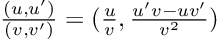
What about quotients? You guessed… the division of dual numbers follows the quotient rule for derivatives:
Last but not least, the power of a dual number to a real number is defined as:
Perhaps you feel curiosity about the multiplication by u’. This corresponds to the chain rule, and enables our dual numbers for something as desirable as function composition.
The operations defined above cover a lot of ground. Indeed, any algebraic operation can be built using them as basic components. This means that we can pass a dual number as the argument of an algebraic function, and here comes the magic, the result will be:
It is hard to overstate how powerful this is. The equation above tells us that just by feeding the function the dual number (x, 1) it will return its value at, plus its derivative! Two for the price of one!
Those readers familiar with complex numbers may find interesting to try the following exercise:
If we define a dual number as
(u, u’) = u + e u’
with e² = 0, all the properties above are automatically satisfied!
Teaching derivatives to your computer
Just as a calculus student will do, the rules of differentiation turn a calculus problem into an algebra one. And the good news: computers are better at algebra than you!
So, how can we implement these rules in a practical way on our computer? Implementing a new object (a dual number) with its own interaction rules sounds like a task for object-oriented programming. And, interestingly enough, the process is surprisingly similar to that of teaching a human student. With the difference that our “digital student” will never forget a rule, apply it the wrong way, or forget a minus sign!
So, how do these rules look, for instance, in Julia? (For a Python implementation, take a look here). First of all, we need to define a Dual object, representing a dual number. In principle, it is as simple as a container for two real numbers:
""" Structure representing a Dual number """
struct Dual
    x::Real
    dx::Real
end
Later, it will come in handy to add a couple of constructors.
""" Structure representing a Dual number """
struct Dual
    x::Real
    dx::Real

    """ Default constructor """
    function Dual(x::Real, dx::Real=0)::Dual
        new(x, dx)
    end

    """ If passed a Dual, just return it
    This will be handy later """
    function Dual(x::Dual)::Dual
        return x
    end
end
Don’t worry too much if you don’t understand the lines above. They have been added only making the Dual object easier to use (for instance, Dual(1) would have failed without the first constructor, and so would have done the application of Dual to a number that is already a Dual).
Another trick that will prove handy soon is to create a type alias for anything that is either a Number (one of Julia's base types) or a Dual.
const DualNumber = Union{Dual, Number}
And now comes the fun part. We’ll teach our new object how to do mathematics! For instance, as we saw earlier, the rule for adding dual numbers is to add both their components, just as in a 2D vector:
import Base: +
function +(self::DualNumber, other::DualNumber)::Dual
    self, other = Dual(self), Dual(other) # Coerce into Dual
    return Dual(self.x + other.x, self.dx + other.dx)
end
We have to teach even more basic stuff. Remember a computer is dramatically devoid of common sense, so, for instance, we have to define the meaning of a plus sign in front of a Dual.
+(z::Dual) = z
This sounds as idiotic as explaining that +3 is equal to 3, but the computer needs to know! Another possibility is using inheritance, but this is an advanced topic beyond the scope of this piece.
Defining minus a Dual will also be needed:
import Base: -
-(z::Dual) = Dual(-z.x, -z.dx)
and actually, it allows us to define the subtraction of two dual numbers as a sum:
function -(self::DualNumber, other::DualNumber)::Dual
	self, other = Dual(self), Dual(other) # Coerce into Dual
	return self + (-other) # A subtraction disguised as a sum!
end
Some basic operations may be slightly trickier than expected. For instance, when is a dual number smaller than another dual number? Notice that in this case, it only makes sense to compare the first elements, and ignore the derivatives:
As we saw before, more interesting stuff happens with multiplication and division:
import Base: *, /

function *(self::DualNumber, other::DualNumber)::Dual
    self, other = Dual(self), Dual(other) # Coerce into Dual
    y = self.x * other.x
    dy = self.dx * other.x + self.x * other.dx # Rule of product for derivatives
    return Dual(y, dy)
end

function /(self::DualNumber, other::DualNumber)::Dual
    self, other = Dual(self), Dual(other) # Coerce into Dual
    y = self.x / other.x
    dy = (self.dx * other.x - self.x * other.dx) / (other.x)^2 # Rule of quotient for derivatives
    return Dual(y, dy)
end
and with potentiation to a real number:
import Base: ^
function ^(self::Dual, other::Real)::Dual
    self, other = Dual(self), Dual(other) # Coerce into Dual
    y = self.x^other.x
    dy = other.x * self.x^(other.x - 1) * self.dx # Derivative of u(x)^n
    return Dual(y, dy)
end
The full list of definitions for algebraic operations is here. For Python, use this link. I recommend taking a look!
After this, each and every time our dual number finds one of the operations defined above in its mysterious journey down a function or a script, it will keep track of its effect on the derivative. It doesn’t matter how long, complicated, or poorly programmed the function is, the second coordinate of our dual number will manage it. Well, as long as the function is differentiable and we don’t hit the machine’s precision… but that would be asking our computer to do magic.
Example
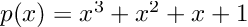
As an example, let’s calculate the derivative of the polynomial:
at x = 3.
For the sake of clarity, we can compute the derivative by hand:
it is apparent that and p(3) = 39 and p’(3) = 34.
Using our Dual object, we can reach the same conclusion automatically:
poly = x -> x^3 + x^2 + x
z = Dual(3, 1)
poly(z)

> Dual(39, 34)
Even if the same polynomial is defined in a more intricate way, the Dual object can keep track:
""" Equivalent to poly = x -> x^3 + x^2 + x
Just uglier """
function poly(x)
	aux = 0 # Initialize auxiliary variable
	for n in 1:3 # Add x^1, x^2 and x^3
		aux = aux + x^n
	end
end

poly(z)

> Dual(39, 34)
What about non-algebraic functions?
The method sketched above will fail miserably as soon as our function contains a non-algebraic element, such as a sine or an exponential. But don’t panic, we can just go to our calculus book and teach our computer some more basic derivatives. For instance, our table of derivatives tells us that the derivative of a sine is a cosine. In the language of dual numbers, this reads:
Confused about the u’? Once again, this is just the chain rule.
The rule of thumb here is, and actually was since the very beginning:
We can create a _factory function that abstracts this structure for us:
function _factory(f::Function, df::Function)::Function
    return z -> Dual(f(z.x), df(z.x) * z.dx)
end
So now, we only have to open our derivatives table and fill line by line, starting with the derivative of a sine, continuing with that of a cosine, a tangent, etc.
import Base: sin, cos

sin(z::Dual) = _factory(sin, cos)(z)
cos(z::Dual) = _factory(cos, x -> -sin(x))(z) # An explicit lambda function is often required
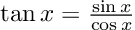
If we know our maths, we don’t even need to fill all the derivatives manually from the table. For instance, the tangent is defined as:
and we already have automatically differentiable sine, cosine, and division in our arsenal. So this line will do the trick:
import Base: tan

tan(z::Dual) = sin(z) / cos(z) # We can rely on previously defined functions!
Of course, hard-coding the tangent’s derivative is also possible, and probably good for code performance and numerical stability. But hey, it’s quite cool that this is even possible!
See a more complete derivatives table here (Python version here).
Example
Let’s compute the derivative of the non-algebraic function
It is easy to prove analytically that the derivative is 1 everywhere (notice that the argument of the tangent is actually constant). Now, using Dual:
fun = x -> x + tan(cos(x)^2 + sin(x)^2)

z = Dual(0, 1)
fun(z)

> Dual(1.557407724654902, 1.0)
Making it more user-friendly
We can use dual numbers to create a user-friendly derivative function:
"""
    derivative(f)

    Seamlessly turns a given function f
    into
    the function's derivative
"""
function derivative(f)
    df = x -> f(Dual(x, 1.0)).dx
    return df
end
Using this, our example above will look like:
fun = x -> x + tan(cos(x)^2 + sin(x)^2)

dfun = derivative(f)
dfun(0)

> 1.0
Another example
Now we want to calculate and visualize the derivatives of:
First, we have to input the function, and the derivative gets calculated automatically:
f(x) = x^2 - 5x + 6 - 5x^3 - 5 * exp(-50 * x^2)

df = derivative(f)
We can visualize the results by plotting a tangent line:
using Plots

I = [-0.7; 0.7]
δ = 0.025
@gif for a = [I[1]:δ:I[2]; I[2]-δ:-δ:I[1]+δ]
    L(x) = f(a) + df(a) * (x - a)
    plot(f, -1, 1, leg=false)
    scatter!([a], [f(a)], m=(:red, 2))
    plot!(L, -1, 1, c=:red)
    ylims!(-5, 15)
end
Is this useful?
Automatic differentiation is particularly useful in the field of Machine Learning, where multidimensional derivatives (better known as gradients) have to be performed as fast and exactly as possible. Said this, automatic differentiation for Machine Learning is usually implemented in a different way, the so-called backward or reverse mode, for efficiency reasons.
A well-established library for automatic differentiation is JAX (for Python). Machine learning frameworks such as Tensorflow and Pytorch also implement automatic differentiation. For Julia, multiple libraries seem to be competing, but Enzyme.jl seems to be ahead. Forwarddiff.jl is also worth taking a look at.
Acknowledgments
I want to say thanks to my colleague and friend Abel Siqueira, for kindly introducing me to Julia and reviewing this post, and to Aron Jansen, for his kind and useful suggestions. A more in-depth introduction can be found in this episode of Chris Rackauckas’ book on scientific machine learning.
The TeX Math Here browser add-in also played an important role: it allowed me to transfer my Latex equations from Markdown to Medium in an (almost) painless way.
I’ll give a brief summary of all my materials here below.
Continuous vs Discrete Differentiation of Solvers
AD of a solver can be done in essentially two different ways: either directly performing automatic differentiation to the steps of the solver, or by defining higher level adjoint rules that will compute the derivative. In some cases these can be mathematically equivalent. For example, forward sensitivity analysis of an ODE $$u’ = f(u,p,t)$$ follows by the chain rule:
then you get $$s = \frac{du}{dp}$$ as the solution to the new equations. So therefore, solve these bigger ODEs and you get the derivative of the solution with respect to parameters as the extra piece. One way to do “automatic differentiation” is to add a derivative rule to the AD library that “if you see ODE solve, then replace the solve with this extended solve and take the latter part as the derivative”. The other way of course is to simply do forward-mode automatic differentiation of the ODE solver library steps itself. It turns out that in this case, if you work out the math the two are mathematically equivalent. Note that it’s not computationally equivalent though since the AD process may SIMD the expressions in a different way, doing some constant folding and common subexpression elimination (CSE) in a way that’s different from the hand-coded version, and thus the performance can be very different even though it’s computationally the same algorithm.
However, there are cases where the “analytical” way of writing the derivative is not equivalent to its automatic differentiation counterpart. For example, the adjoint method is a different way to get $$\frac{du}{dp}$$ values in $$\mathcal{O}(n+p)$$ time (instead of the $$\mathcal{O}(np)$$ time of the forward sensitivities above) by solving an ODE forward and some related ODE backwards (for a full derivation and description, see the lecture notes or the recorded video). If you were to do reverse-mode automatic differentiation of the solver, you do not get a mathematically equivalent algorithm. For example, if the solver for the ODE was Euler’s method, reverse-mode AD would be mathematically equivalent to solving the forward ODE with Euler’s method and the reverse ODE with something like implicit Euler (where part of the implicit equation is solved exactly using a cached value from the forward solve).
So What is Better, Continuous Derivative Rules or Discrete Derivatives of the Solver?
Forward-mode outperforms reverse-mode / adjoint techniques when the equations are “sufficiently small”. For modern implementations this seems to be at around 100.
For forward-mode cases, “good” automatic differentiation libraries can make use of structure between the primal and derivative constructions to better CSE/SIMD the generated code for the derivative term, thus forward-mode AD of the solver can be much faster than forward sensitivity analysis even though the two are mathematically the same operation.
For reverse-mode cases, the continuous adjoints seem to be faster with current implementations.
But that last bit then has many caveats to put on it. For one, there seems to be a trade-off between performance and stability here. This is noted in the appendix of the paper “Universal Differential Equations for Scientific Machine Learning, which states:
Previous research has shown that the discrete adjoint approach is more stable than continuous adjoints in some cases [53, 47, 94, 95, 96, 97] while continuous adjoints have been demonstrated to be more stable in others [98, 95] and can reduce spurious oscillations [99, 100, 101]. This trade-off between discrete and continuous adjoint approaches has been demonstrated on some equations as a trade-off between stability and computational efficiency [102, 103, 104, 105, 106, 107, 108, 109, 110]. Care has to be taken as the stability of an adjoint approach can be dependent on the chosen discretization method [111, 112, 113, 114, 115]
with the references pointing to those in the manuscript.
This is discussed in even more detail in the manuscript Stiff Neural Ordinary Differential Equations which showcases how there are many ways to implement “the adjoint method”, and they can have major differences in stability, essentially trading off memory or performance for improved stability properties.
Special Case: Implicit Equations
The above discussion shows that there are good reasons to differentiate solvers directly, and good reasons to instead write derivative rules for solvers which use forward/adjoint equations. For time series equations, this always has a trade-off. There is an important special case here though that for methods which iterate to convergence, automatic differentiation of the solver is essentially never a good idea. The reason is because the implicit function theorem gives that the derivative of the solution is directly defined at the solution point. For example, for solving $$f(x,p) = 0$$, if $$x^\ast$$ is the value of $$x$$ which satisfies the equation, then $$\frac{d x^\ast}{dp} = …$$. In other words, Newton’s method might take $$n$$ steps, and thus automatic differentation will need to differentiate $$f$$ at least $$n$$ times. But if you use the implicit function theorem result, then you only need to differentiate it once!
Note of course a similar performance vs stability trade-off does apply here. Since this derivation assumes you have $$x^\ast$$ such that $$f(x^\ast,p) = 0$$ exactly, but you don’t. Newton’s method from the solve will give you something that satisfies the equation to tolerance, so maybe $$f(x^\ast,p) \approx 10^{-8}$$, which means that the derivative expression is also only approximate, and this then induces an error in the gradient etc. Thus direct differentiation of Newton’s method can be more accurate, and you need to worry about tolerance here if the gradients seem sufficiently off.
Does Differentiation of Solver Internals Make Sense or Have a Meaning?
“ODE solvers” have all sorts of things in there, like adaptivity parameters and heuristics. One of the things that happens when you do automatic differentiation of the solver is that you aren’t just differentiating the solver’s states and parameters, but the process will differentiate everything. It turns out that AD of a solver can thus be useful in some tricky ways which put this to use. For example, at ICML we had a paper which regularized the parameters of a neural ODE by the sum of the computed error estimates of the adaptivity heuristics. This would then push the learned equation towards an area of parameter space where the adaptivity gives the largest time steps possible, and thus the learned equation is the “fastest possible learned equation that fits the time series”. Such a trick is only possible if you are doing automatic differentiation of the solver since you’d need to differentiate the solver’s internals in order to have access to those values in the loss function! This just shows one of many ways in which AD’s “extra information” which analytical continuous derivative definitions don’t have could potentially be useful for some applications.
Automatic Differentiation in Continuous Sensitivity Methods
Finally, I want to note that even when you attempt to avoid automatic differentiation of the solver by using continuous sensitivity methods, it turns out that the optimal way to build the extended equations is to use automatic differentiation!
Summary: there are many good reasons to do automatic differentiation of solvers, but there are also many good reasons to use some analytical derivative techniques. But even if you do analytical derivative techniques, you still want to automatic differentiate something in order to do it optimally!
For example, let’s return to the forward sensitivity equations:
It turns out that $$\frac{df}{du} s$$ does not require computing the full Jacobian. This operation, known as Jacobian-vector products or jvps, are the primitive operation of forward-mode automatic differentiation and thus special seeding of a forward-mode AD tool gives a faster and more robust algorithm than a finite difference form. When done correctly, this operation is computed without ever building the full Jacobian. A trick for this does exist in the finite difference sense as well:
$$\frac{df}{du} s \approx \frac{f(u + \epsilon s) – f(u)}{\epsilon}$$
In the same vein, continuous adjoints of ODE solves boil down to defining a differential equation which is solved backwards and that differential equation which is solved backwards has a term which is $$\frac{df}{du}^T s$$, i.e. Jacobian transposed times a vector, also known as the vector-Jacobian product because it’s equivalent to $$s^T \frac{df}{du}$$ when transposed. It turns out that this is the primitive operation of reverse-mode AD, which then allows for computing this operation without fully building the Jacobian. There is no analogue for this operation with finite differencing, which means that there’s a pretty massive performance gain from doing this properly. Our paper A Comparison of Automatic Differentiation and Continuous Sensitivity Analysis for Derivatives of Differential Equation Solutions measures this effect on a stiff partial differential equation, getting:
The takeaway from this plot is that using these AD tricks results in a few orders of magnitude performance improvements (by avoiding the Jacobian construction, which are the “seeding” versions on the left, the right shows the difference that different AD techniques make, which itself is another few orders of magnitude). When people note that the Julia differential equation adjoint solvers are much faster than the adjoints from Sundials COVDES and IDAS on large equations, this part right here is one of the major factors because Sundials does not embed a reverse AD engine into its adjoint code to do the vjp definitions, and instead falls back to using a numerical formulation unless the user provides a vjp override, which is seemingly to be uncommon to do but from these plots clearly should be done more often.
Summary
In total, what can we takeaway so far about differentiating solvers?
There are some advantages to differentiating solvers, but there are also some advantages to mixing in analytical continuous adjoints. It’s context-dependent which is better.
Even when mixing in analytical continuous derivative rules, these are best defined with automatic differentiation within their constructed equations, so one cannot avoid AD completely if one wishes to achieve full performance on arbitrary models.
For cases which converge to some kind of implicitly defined solution, using special adjoint tricks will be much better than direct differentiation of the solver.
There’s still a lot more to mention, especially as stochastic simulation gets involved, but I’ll cut this here for now. As you can see, there’s still some open questions that are being investigated in the field, so if you find this interesting please feel free to get in touch.