Author Archives: Christian Groll

Downloading SP500 stock price data with Julia

By: Christian Groll

Re-posted from: http://grollchristian.wordpress.com/2014/09/05/sp500-data-download-julia/

In a previous post I already described how to download stock price data for all constituents of the SP500 with R. Meanwhile, however, I shifted all of my coding to the new and very promising technical computing language julia. I obviously wanted to also enjoy the convenience of downloading stock price data directly in julia. Hence, in this post I will describe how one could use julia to download stock price data from Yahoo!Finance in general, and – as an advanced use case – how to download adjusted closing prices for all SP500 constituents. We also will make use of julia’s parallel computing capabilities, in order to tremendously speed up the downloading and processing steps compared to my original code in R.

Before we start, we first need to make sure that we have all relevant packages installed. As a format for storing time series data I always rely on the TimeData package from the official package repository:

Pkg.add("TimeData")

The functions required for data download are bundled in the not yet registered EconDatasets package, which we can clone from github:

Pkg.clone("https://github.com/JuliaFinMetriX/EconDatasets.jl.git")

1 Download data using readYahooFinance

Now that all required packages are installed, we will first demonstrate a simple use case for the low-level function readYahooFinance. This functions allows easy access to the complete stock data provided by Yahoo!Finance, comprising fields open, high, low, close, volume and adjusted close. As an example, we now download data for NASDAQ-100, S&P 500 and EURO STOXX 50 Index.

using TimeData
using Dates
using EconDatasets

tickerSymbs = ["^NDX"
               "^GSPC"
               "^STOXX50E"]


dates = Date(1960,1,1):Date(2014,7,20)

indexData = [readYahooFinance(dates, symb) for symb in tickerSymbs]

## display first five dates of NASDAQ
indexData[1][1:5, :]

idx Open High Low Close Volume Adj_Close
1985-10-01 221.24 224.32 221.13 224.28 153160000 112.14
1985-10-02 224.28 225.08 221.56 221.65 164640000 110.82
1985-10-03 221.68 222.37 220.24 221.74 147300000 110.87
1985-10-04 221.74 221.74 219.71 220.15 147900000 110.07
1985-10-07 220.15 220.27 216.35 216.4 128640000 108.2

Using comprehension, the function readYahooFinance can be applied to all ticker symbols in an Array. The output will be an Array of type Any, with individual entries being of type Timematr.

When we focus on one variable for each stock only, we can store the data more concisely in a single TimeData object. Therefore, we join individual stocks at the their idx entries. We do not want to lose any data at this step, so that we will use an outer join in order to get a row for each date that occurs for at least one of the individual stocks. Missing values will be replaced by NA, so that we now get an object of type Timenum, as Timematr objects are not allowed to contain NAs.

adjCloseData = indexData[1][:Adj_Close]
names!(adjCloseData.vals, [symbol(tickerSymbs[1])])

for ii=2:3
    nextStock = indexData[ii] |>
         x -> x[:Adj_Close]
    names!(nextStock.vals, [symbol(tickerSymbs[ii])])
    adjCloseData = joinSortedIdx_outer(adjCloseData, nextStock)
end

adjCloseData[[1:10; (end-10):end], :]

idx ^NDX ^GSPC ^STOXX50E
1950-01-03 NA 16.66 NA
1950-01-04 NA 16.85 NA
1950-01-05 NA 16.93 NA
1950-01-06 NA 16.98 NA
1950-01-09 NA 17.08 NA
1950-01-10 NA 17.03 NA
1950-01-11 NA 17.09 NA
1950-01-12 NA 16.76 NA
1950-01-13 NA 16.67 NA
1950-01-16 NA 16.72 NA
2014-07-04 NA NA 3270.47
2014-07-07 3910.71 1977.65 3230.92
2014-07-08 3864.07 1963.71 3184.38
2014-07-09 3892.91 1972.83 3203.1
2014-07-10 3880.04 1964.68 3150.59
2014-07-11 3904.58 1967.57 3157.05
2014-07-14 3929.46 1977.1 3185.86
2014-07-15 3914.46 1973.28 3153.75
2014-07-16 3932.33 1981.57 3202.94
2014-07-17 3878.01 1958.12 3157.82
2014-07-18 3939.89 1978.22 3164.21

2 Download adjusted closing prices of SP500 constituents

Now that we already have seen a first use case of function readYahooFinance, we now want to try the capabilities of julia and the EconDatasets package with a more challenging task. Hence, we want to download adjusted stock prices for all constituents of the SP500 in a fully automated way. Therefore, we first need to get a list of the ticker symbols of all constituents, which we can get from the S&P homepage. However, this list is stored as an Excel sheet with .xls extension, and we need to read in this binary file with package Taro.

To make Taro work, you first need to make sure that it is able to find Java on your system. If your path deviates from the default settings, just make sure to set the respective JAVA_LIB environment variable in your .bashrc file. In my case, the variable is set as follows:

# 64-bit machine
# JAVA_LIB="/usr/lib/jvm/java-7-openjdk-amd64/jre/lib/amd64/server/"

# 32-bit machine
JAVA_LIB="/usr/lib/jvm/java-7-openjdk-i386/jre/lib/i386/server/"
export JAVA_LIB

We can now install and load package Taro:

Pkg.add("Taro")

using Taro
Taro.init()

Found libjvm @ /usr/lib/jvm/java-7-openjdk-i386/jre/lib/i386/server/

If something with your Taro configuration is not correct, you will get an error at this step. In this case, you could simply download and export the Excel sheet to .csv manually, which you then can read in with function readtable from the DataFrames package.

Otherwise, you can use Taro to download and read in the respective part of the Excel sheet:

url = "http://us.spindices.com/idsexport/file.xls?hostIdentifier=48190c8c-42c4-46af-8d1a-0cd5db894797&selectedModule=Constituents&selectedSubModule=ConstituentsFullList&indexId=340"
filepath = download(url)
constituents = Taro.readxl(filepath, "Constituents", "A10:B511")
head(constituents)

Constituent Symbol
3M Co MMM
Abbott Laboratories ABT
AbbVie Inc. ABBV
Accenture plc ACN
ACE Limited ACE
Actavis plc ACT

We now should have name and ticker symbol of each SP500 constituent stored as a DataFrame. In my case, however, there even is one ticker symbol too much, although I do not know why:

(nTicker, nVars) = size(constituents)

501
2

An inconsistency that I will not further invest at this point. In addition, however, some of the ticker symbols are automatically read in as boolean values, and we will have to convert them to strings first. Let’s display all constituents with boolean values:

isBoolTicker = [isa(tickerSymbol, Bool) for tickerSymbol in
                constituents[:Symbol]]

constituents[find(isBoolTicker), :]

Constituent Symbol
AT&T Inc true
Ford Motor Co false

The reason for this is that the respective ticker symbols are “T” and “F”, which will be interpreted as boolean values. Once we did correct for this mistake, we transform the array of ticker symbols into an Array of type ASCIIString.

indTrue = find(constituents[2] .== true)
indFalse = find(constituents[2] .== false)

constituents[indTrue, 2] = "T"
constituents[indFalse, 2] = "F"

tickerSymb = ASCIIString[constituents[:Symbol]...]
tickerSymb[1:5]

MMM
ABT
ABBV
ACN
ACE

Now that we already have a list of all ticker symbols, in principle we could apply the same procedure as before: download each stock, extract the adjusted closing prices, and join all individual price series. However, as we have 500 stocks, this procedure would already take approximately 15 minutes if each individual stock took only 2 seconds. Hence, we strive for a much faster result using julia’s parallel computing capabilities, and this is already implemented as function readYahooAdjClose.

Under the hood, readYahooAdjClose uses a map-reduce structure. As the map step, for any given ticker symbol we download the data, extract the adjusted closing prices and rename the column to its ticker symbol. As reduce step we need to specify some operation that combines the individual results of the map step – in our case, this is function joinSortedIdx_outer.

Let’s now set the stage for parallel computation, add three additional processes and load the required packages on each process.

addprocs(3)

@everywhere using Dates
@everywhere using DataFrames
@everywhere using TimeData
@everywhere using EconDatasets

3-element Array{Any,1}:
 2
 3
 4

To run the parallelized code, simply call function readYahooAdjClose:

dates = Date(1960,1,1):Date(2014,7,20)

## measure time
t0 = time()

@time vals = readYahooAdjClose(dates, tickerSymb, :d)

t1 = time()
elapsedTime = t1-t0
mins, secs = divrem(elapsedTime, 60)

Downloading of all 500 stocks did only take:

println("elapsed time: ", int(mins), " minutes, ", ceil(secs), " seconds")

elapsed time: 3 minutes, 45.0 seconds

Now we convert the data of type Timedata to type Timenum and store the result in the EconDatasets data directory:

valsTn = convert(Timenum, vals)
pathToStore = joinpath(Pkg.dir("EconDatasets"), "data", "SP500.csv")
writeTimedata(pathToStore, valsTn)

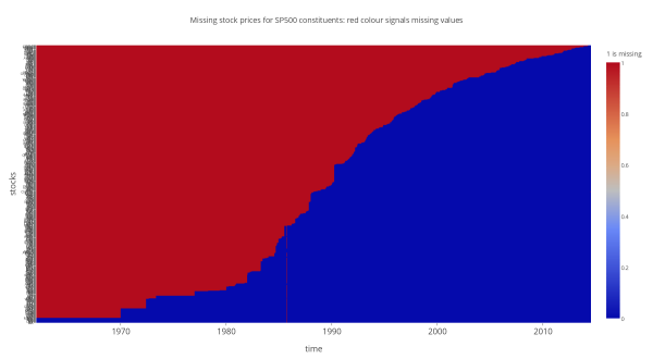
3 Visualize missing values

From previous experiences I already know that the saying “you get what you pay for” also holds for the free Yahoo!Finance database: the data comes with a lot of missing values. In order to get a feeling for the data quality, we want to visualize all missing values. Therefore, we sort all assets with respect to the number of missing values.

(nObs, nStocks) = size(valsTn)

NAorNot = Array(Int, nObs, nStocks)

for ii=1:nStocks
    NAorNot[:, ii] = isna(vals.vals[ii])*1
end

nNAs = sum(NAorNot, 1)
p = sortperm(nNAs[:])
tickSorted = tickerSymb[p]
NAorNotSorted = NAorNot[:, p]

For the visualization, we rely on plot.ly, as we get an interactive graphic this way. This allows the identification of individual stocks in the graphic by simple mouse clicks. If you want to replicate the figure, you will need to sign in with an own and free plot.ly account.

Pkg.clone("https://github.com/plotly/Plotly.jl")
using Plotly

## sign in with your account
## Plotly.signin("username", "authentication")

nToPlot = nStocks
datsStrings = ASCIIString[string(dat, " 00:00:00") for dat in valsTn.idx]
data = [
        [
         "z" => NAorNotSorted[:, 1:nToPlot],
         "y" => tickSorted[1:nToPlot],
         "x" => datsStrings, 
         "type" => "heatmap"
         ]
        ]

response = Plotly.plot([data], ["filename" => "Published graphics/SP500 missing values", "fileopt" => "overwrite"])
plot_url = response["url"]

Although the resulting graphic easily could be directly embedded into this html file, you will need to follow this link to watch it, since the plot.ly graphic is a large data file and hence takes quite some time to load. Nevertheless, I also exported a .png version of the graphic, which you can find below. Thereby, red dots are representing missing values.

missing_values.png

4 Get logarithmic returns

So now we already have our closing price data at our hands. However, in financial econometrics we usually analyze return data, as prices are non-stationary almost always. Hence, we now want to derive returns from our price series.

For this step I rely on the also not yet registered Econometrics package:

Pkg.clone("https://github.com/JuliaFinMetriX/Econometrics.jl.git")
using Econometrics

The reason for this is that I can make use of function price2ret then, which implements a slightly more sophisticated approach to return calculation. This can best be described through an example, which we can set up using function testcase from the TimeData package:

logPrices = testcase(Timenum, 4)

idx prices1 prices2
2010-01-01 100 110
2010-01-02 120 120
2010-01-03 140 NA
2010-01-04 170 130
2010-01-05 200 150

As you can see, the example logarithmic prices have a single missing observation at January 3rd. Straightforward application of the logarithmic return calculation formula hence will result in two missing values in the return series:

logRetSimple = logPrices[2:end, :] .- logPrices[1:(end-1),:]

idx prices1 prices2
2010-01-02 20 10
2010-01-03 20 NA
2010-01-04 30 NA
2010-01-05 30 20

In contrast, function price2ret assumes that single missing values in the middle of a price series are truly non-existent: there is no observation, because the stock exchange was closed and there simply was no trading. For example, this could easily happen if you have stocks from multiple countries with different holidays. Note, that this kind of missingness is different to a case where the stock exchange was open and trading did occur, but we were not able to observe the resulting price (for a more elaborate discussion on this point take a look at my blog post about missing stock price data). Using function price2ret, you ultimately will end up with a stock return series with only one NA for this example:

## get real prices
logRetEconometrics = price2ret(logPrices; log = true)

idx prices1 prices2
2010-01-02 20 10
2010-01-03 20 NA
2010-01-04 30 10
2010-01-05 30 20

So the final step in our logarithmic return calculation is to apply price2ret to the logarithmic prices, specify the usage of differences for return calculations through log = true, and multiply the results by 100 in order to get percentage returns.

percentLogRet = price2ret(log(valsTn); log = true).*100

Alternatively, you could get discrete returns with:

percentDiscRet = price2ret(valsTn; log = false).*100

Filed under: financial econometrics, Julia Tagged: data, sp500

IJulia on Amazon EC2 instance

By: Christian Groll

Re-posted from: http://grollchristian.wordpress.com/2014/09/01/ijulia-for-amazon-ec2/

In this blog post I want to give a description of how to set up a running IJulia server on an Amazon EC2 instance. Although there already are some useful resources on the topic out there, I didn’t find any comprehensive tutorial yet. Hence, I decided to write down my experiences, just in case it might be a help for others.

1 What for?

At this point, you might think: “okay – but what for?”. Well, what you get with Amazon AWS is a setting where you can easily load a given image on a computer that can be chosen from a range of different memory and processing characteristics (you can find a list of available instances here). In addition, you can also store some private data on a separate volume with Amazon’s Elastic Block Store. So taking both components together, this allows fast setup of the following workflow:

  • choose a computer with optimal characteristics for your task
  • load your ready-to-go working environment with all relevant software components pre-installed
  • mount an EBS volume with your private data

And your customized computer is ready for work!

So, what you get is a flexible environment that you can either use for selected tasks with high computational requirements only, or that you steadily use with a certain baseline level of CPU performance and only scale it up when needed. This way, for example, you could outsource computations from your slow netbook to the Amazon cloud whenever the weather allows you to do your work outside in your garden. Any easy to transport and lightweight netbook already provides you with an entrance to huge computational power in the Amazon cloud. However, compared to a moderately good local computer at home, it doubt that the Amazon cloud will be a cost-efficient alternative for permanent work yet. Besides, you always have the disadvantage of having to rely on a good internet connection, which especially becomes problematic when traveling.

Anyways, I am sure you will find your own use cases for IJulia in the cloud, so let’s get started with the setup.

2 Setting up an Amazon AWS account

The first step, of course, is setting up an account at Amazon web services. You can either log in with an existing Amazon account, or just create a completely new account from scratch. At this step, you will already be required to leave your credit card details. However, Amazon automatically provides you with a free usage tier, comprising (among other benefits) 750 hours of free EC2 instance usage, as well as 30 GB of EBS storage. For more details, just take a look at Amazon’s pricing webpage.

3 Setting up an instance

Logging in to your account will take you to the AWS Management Console: a graphical user interface that allows managing all of your AWS products. Should you plan on making some of your products available to other users as well (employees, students, …), you could easily assign rights to groups and users through their AWS Identity and Access Management (IAM), so that you are the only person with access to the full AWS Management Console.

Now let’s create a new instance. In the overview, click on EC2 to get to the EC2 Dashboard, where you can manage and create Amazon computing instances. You need to specify the region where your instance should physically be created, which you can select in the upper right corner. Then, click on instances on the left side, and select Launch Instance to access the step by step instructions.

In the first step you need to select a basic software equipment that your instance should use. This determines your operating system, but also could comprise additional preinstalled software. You can select from a range of Amazon Machine Images (AMI), which could be images that are put together either by Amazon, by other members of the community or by yourself. At the end of the setup, we will save our preinstalled IJulia server as AMI as well, so that we can easily select it as ready-to-go image for future instances. For now, however, we simply select an image with a basic operating system installed. For the instructions described here, I select Ubuntu Server 14.04 LTS.

In the next step we now need to pick the exact memory and processing characteristics for our instance. For this basic setup, I will use a t2.micro instance type, as it is part of the free usage tier in the first 12 months. If you wanted to use Amazon EC2 for computationally demanding tasks, you would select a type with better computational performance.

In the next two steps, Configure Instance and Add Storage, I simply stick with the default values. Only in step 5 I manually add some tags to the instance. Tags can be added as key-value pairs. So, for example, we could use the following tags to describe our instance:

  • task = ijulia,
  • os = ubuntu,
  • cpu = t2.micro

By now, all characteristics of the instance itself are defined, and we only need to determine the traffic that is allowed to reach our instance. In other words: we have defined a virtual computer in Amazon’s cloud – but how can we communicate with it?

In general, there are several ways to access a remote computer. The standard way on Linux computers would be through a terminal with SSH connection. This way, we can execute commands at the remote computer, which allows the installation of software, for example. In addition, however, we might want to communicate with the remote computer through other channels than the terminal. For example, in our case we want to access the computing power of the remote through an IJulia tab in our browser. Hence, we need to determine all ways through which a communication to the remote should be allowed. For security reasons, you want to keep these communication channels as sparse and restricted as possible. Still, you need to allow some of these channels in order to use our instance in the manner that you want to. In our case, we add a new rule that allows access to our instance through the browser, and hence select All TCP as its type. Be warned, however, that I am definitely not an expert on computer security issues, so that this rule might be overly permissive. Ultimately, you only want to permit communication through https with a given port (8998 in our example), and there might be better ways to achieve this. Still, I will add an additional layer of protection by restricting permission to my current IP only. If you do this, however, then you most likely need to adapt your settings each time that you restart your computer, as your IP address might change. Anyways, in many cases your instance will only live temporarily, and will be deleted after completion of a certain task. Your security concerns for such a short-living instance hence might be rather limited. Either way, you can store your current settings as a new security group, so that you can select the exact same settings for some of your future instances. I will choose “IJulia all tcp” as name of the group.

Once you are finished with your security settings, click Review and Launch and confirm your current settings with Launch. This will bring up a dialogue that lets you exchange ssh keys between remote computer and local computer. You can either create a new key pair or choose an already existing pair. In any case, make sure that you will really have access to the chosen key afterwards, because it will be the only way to get full access to your remote. If you create a new pair, the key will automatically be downloaded to your computer. Just click Launch Instance afterwards, and your instance will be available in a couple of minutes.

4 Installing and configuring IJulia

Once your instance will be displayed as running you can connect to it through ssh. Therefore, we need to use the ssh key that we did get during the setup, which I stored in my download folder with name aws_ijulia_key.pem. First, however, we will need to change the permissions of the key, so that it can not be accessed by everyone. This step is mandatory – otherwise the ssh connection will fail.

chmod 400 ~/Downloads/aws_ijulia_key.pem

Now we are ready to connect. Therefore, we need to link to the ssh key through option -i. The address of your instance is composed of two parts. First, the username, which is ubuntu for the case of an Ubuntu operating system. And second, we need to copy the Public DNS of the instance, which we can find listed in the description when we select the instance in the AWS Management Console.

ssh -i ~/Downloads/aws_ijulia_key.pem 
   ubuntu@ec2-54-76-169-215.eu-west-1.compute.amazonaws.com

Now that we have access to a terminal within our instance, we can use it to install all required software components for IJulia. First, we install Julia from the julianightlies repository.

sudo add-apt-repository ppa:staticfloat/julia-deps
sudo add-apt-repository ppa:staticfloat/julianightlies
sudo apt-get update
sudo apt-get -y install julia

We now already could use Julia through the terminal. Then we need to install a recent version of ipython, which we can do using pip.

sudo apt-get -y install python-dev ipython python-pip
sudo pip install --upgrade ipython

IJulia also requires some additional packages:

sudo pip install jinja2 tornado pyzmq

At last, we need to install the IJulia package:

julia -e 'Pkg.add("IJulia")'

At this step, we have installed all required software components, which we now only need to configure correctly.

The first thing we need to do is set up a secure way of connecting to IJulia through our browser. Therefore, we need to set a password that we will be required to type in when we log in. We will create this password within ipython. To start ipython on your remote, type

ipython

Within ipython, type the following

from IPython.lib import passwd
passwd()

Now type in your password. For this demo, I chose ‘juliainthecloud’, equal to the setup here. IPython then prints out the encrypted version of this password, which in my case is

'sha1:32c75aa1c075:338b3addb7db1c3cb2e10e7b143fbc60be54c1be'

You will need this hashed password later, so you should temporarily store it in your editor.

We now can exit ipython again:

exit

As a second layer of protection, we need to create a certificate which our browser will automatically use when it communicates with our IJulia server. This way, we will not have to send our password in plain text to the remote computer, but the connection will be encrypted right away. In your remote terminal, type:

mkdir ~/certificates
cd ~/certificates
openssl req -x509 -nodes -days 365 -newkey rsa:1024 -keyout 
   mycert.pem -out mycert.pem

You are asked to add some additional information to your certificate, but you can also skip all fields by pressing enter.

Finally, we now only need to configure IJulia. Therefore, we add the following lines to the julia profile within ipython. This profile should already have been created through the installation of the IJulia package, so that we can open the respective file with vim:

vim ~/.ipython/profile_julia/ipython_notebook_config.py

Press i for insert mode, and after

c = get_config()

add the following lines (which I myself did get from here):

# Kernel config
c.IPKernelApp.pylab = 'inline'  # if you want plotting support always
# Notebook config

c.NotebookApp.certfile = u'/home/ubuntu/certificates/mycert.pem'
c.NotebookApp.ip = '*'
c.NotebookApp.open_browser = False
c.NotebookApp.password = 
   u'sha1:32c75aa1c075:338b3addb7db1c3cb2e10e7b143fbc60be54c1be'

# It is a good idea to put it on a known, fixed port
c.NotebookApp.port = 8998

Make sure that you did set c.NotebookApp.password to YOUR hashed password from before.

To leave vim again, press escape to end insert mode and :wq to save and quit.

5 Starting and connecting to IJulia server

We are done with the configuration, so that we now can connect to our IJulia server. To start the server on the remote, type

sudo ipython notebook --profile=julia
# nohup ipython notebook  --profile julia > ijulia.log &

And to connect to your server, open a browser on your local machine and go to

https://ec2-54-76-169-215.eu-west-1.compute.amazonaws.com:8998

This will pop up a warning that the connection is untrust. Don’t worry, this is just because we are using the encryption that we did set up ourselves, and this certificate is not officially registered. Once you allow the connection, an IJulia logo appears, and you will be prompted for your password.

Note, however, that the Public DNS of your instance changes whenever you stop your instance from running. Hence, you need to type a different URL when you connect to IJulia the next time.

6 Store as AMI

Now that we have done all this work, we want to store the exact configuration of our instance as our own AMI to be able to easily load it on any EC2 instance type in the future. Therefore, we simply stop our running instance in the AWS Management Console (after we also stopped the running IJulia server of course). Right-click on it as soon as the Instance State says stopped. Choose create image, select an appropriate name for your configuration, and you’re done. The next time you launch a new image, you can simply select this AMI instead of the Ubuntu 14.04 AMI that we did use previously.

However, creating an image of your current instance requires you to store a snapshot of your volume in your elastic block store, which might cause additional costs depending on your AWS profile. Using Amazon’s free usage tier, you have 1GB free snapshot storage at your disposal. Due to compression, your snapshot should be smaller in storage size than the original 8GB of your volume. Nevertheless, I do not yet know where to look up the overall storage size of my snapshots (determining the size of individual snapshots if you have multiple snapshots is even impossible). I only can say that Amazon did not bill me for anything yet, so I assume that the snapshot’s size should be smaller than 1GB.

7 Add volume

In order to have your data available for multiple instances, you should store it on a separate volume, which then can be attached to any instance you like. This also allows easy duplication of your data, so that you can attach one copy of it to your steadily running t2.micro instance, while the other one gets attached to some temporary instance with greater computational power in order to perform some computationally demanding task.

For creation and mounting of a data volume we largely follow the steps shown in the documentation.

On the left side panel, click on Volumes, then select Create Volume. As size we choose 5 GB, as this should leave us with enough free storage size in order to simultaneously run two instances, each with its own copy of personal data mounted. Also, we choose to not encrypt our volume, as t2.micro instances do not support encrypted volumes.

Now that the volume is created, we need to attach it to our running instance. Right-click on the volume and select Attach Volume. Type in the ID of your running instance, and as your device name choose /dev/sdf as proposed for linux operating systems.

Connect to your running instance with ssh, and display all volumes with the lsblk command in order to find the volume name. In my case, the new attached volume displays as xvdf. Now, since we created a new volume from scratch, we additionally need to format it. Be careful to not conduct this step if you attach an already existing volume with data, as it would delete all of your data! For my volume name, the command is

sudo mkfs -t ext4 /dev/xvdf

The device can now be mounted anywhere in your file system. Here we will mount it as folder research in the home directory.

sudo mkdir ~/research
sudo mount /dev/xvdf /home/ubuntu/research

And, in case you need it at some point, you can unmount it again with

umount -d /dev/xvdf

8 Customization

Well, now we know how to get an IJulia server running. To be honest, however, this really is only half of the deal if you want to use it for more than just some on-the-fly experimenting. For more elaborate work, you need to be able to also conveniently perform the following operations at your Amazon remote instance:

  • editing files on the remote
  • copying files to and from the remote

There are basically two ways that allow you to edit files on the remote. First, you use some way of editing files directly through the terminal. For example, you could open a vim session in your terminal on the remote itself. Second, you work with a local editor that allows to access files on a remote computer via ssh. As emacs user, I stick with this approach, as emacs tramp allows working with remote files as if they were local.

For synchronization of files to the remote I use git, as I host all of my code on github and bitbucket. However, I also want my remote to communicate with my code hosting platforms through ssh without any additional password query. In principle, one could achieve this through the standard procedure: creating a key pair on the remote, and copying the public key to the respective file hosting platform. However, this could become annoying, given that we have to perform it whenever we launch a new instance in the future. There is a much easier way to enable communication between remote server and github / bitbucket: using SSH agent forwarding. What this does, in simple terms, is passing your local ssh keys on to your remote computer, which is then allowed to use them for authentication itself. To set this up, we have to add some lines to ./ssh/config (take a look at this post for some additional things that you could achieve with your config file). And since we are already editing the file, we also take the chance to set an alias aws_julia_instance for our server and automatically link to the required login ssh key file. Our config file now is

Host aws_julia_instance
     HostName ec2-54-76-169-215.eu-west-1.compute.amazonaws.com
     User ubuntu
     IdentityFile ~/Downloads/aws_ijulia_key.pem
     ForwardAgent yes

Remember: you have to change the HostName in your config file whenever you stop your instance, since the Public DNS changes.

Given the settings in our config file, we now can access our remote through ssh with the following simple command:

ssh aws_julia_instance

And, given that we have set up ssh access to github and bitbucket on our local machine, we can use these keys on the remote as well.

As a last convenience for the synchronization of files on your remote I recommend the use of myrepos, which allows you to easily keep track of all modifications in a whole bunch of repositories. You can install it with

mkdir ~/programs
cd ~/programs
git clone https://github.com/joeyh/myrepos.git
cd /usr/bin/
sudo ln -s ~/programs/myrepos/mr

Filed under: Julia, tools Tagged: amazon, aws, ec2, ijulia, Julia

Coping with missing stock price data

By: Christian Groll

Re-posted from: http://grollchristian.wordpress.com/2014/08/13/missing-data/

1 Missing stock price data

When downloading historic stock price data it happens quite frequently that some observations in the middle of the sample are missing. Hence the question: how should we cope with this? There are several ways how we could process the data, each approach coming with its own advantages and disadvantages, and we want to compare some of the most common approaches in this post.

In any case, however, we want to treat missing values as NA and not as Julia’s built-in NaN (a short justification on why NA is more suitable can be found here). Hence, data best should be treated through DataFrames or – if the data comes with time information – through type Timenum from the TimeData package. In the following, we will use these packages in order to show some common approaches to deal with missing stock price data using an artificially made up data set that shall represent logarthmic prices.

The reason why we are looking at logarthmic prices and returns instead of normal prices and net returns is just that logarithmic returns are defined as simple difference between logarithmic prices of successive days:

\displaystyle r_{t}^{\log}=\log(P_{t}) - \log(P_{t-1})

This way, our calculations simply involve nicer numbers, and all results equally hold for normal prices and returns as well.

We will be using the following exemplary data set of logarthmic prices for the comparison of different approaches:

using TimeData
using Dates
using Econometrics

df = DataFrame()
df[:stock1] = @data([100, 120, 140, 170, 200])
df[:stock2] = @data([110, 120, NA, 130, 150])

dats = [Date(2010, 1, 1):Date(2010, 1, 5)]

originalPrices = Timenum(df, dats)
idx stock1 stock2
2010-01-01 100 110
2010-01-02 120 120
2010-01-03 140 NA
2010-01-04 170 130
2010-01-05 200 150

One possible explanation for such a pattern in the data could be that the two stocks are from different countries, and only the country of the second stock has a holiday at January the 3rd.

Quite often in such a situation, people just refrain from any deviations from the basic calculation formula of logarithmic returns and calculate the associated returns as simple differences. This way, however, each missing observation NA will lead to two NAs in the return series:

simpleDiffRets = originalPrices[2:end, :] .- originalPrices[1:(end-1), :]
idx stock1 stock2
2010-01-02 20 10
2010-01-03 20 NA
2010-01-04 30 NA
2010-01-05 30 20

For example, this also is the approach followed by the PerformanceAnalytics package in R:

library(tseries)
library(PerformanceAnalytics)

stockPrices1 <- c(100, 120, 140, 170, 200)
stockPrices2 <- c(110, 120, NA, 130, 150)

## combine in matrix and name columns and rows
stockPrices <- cbind(stockPrices1, stockPrices2)
dates <- seq(as.Date('2010-1-1'),by='days',length=5)
colnames(stockPrices) <- c("A", "B")
rownames(stockPrices) <- as.character(dates)
(stockPrices)

returns = Return.calculate(exp(stockPrices), method="compound")
nil nil
20 10
20 nil
30 nil
30 20

When we calculate returns as the difference between successive closing prices P_{t} and P_{t-1}, a single return simply represents all price movements that happened at day t, including the opening auction that determines the very first price at this day.

Thinking about returns this way, it obviously makes sense to assign a value of NA to each day of the return series where a stock exchange was closed due to holiday, since there simply are no stock price movements on that day. But why would we set the next day’s return to NA as well?

In other words, we should distinguish between two different cases of NA values for our prices:

  1. NA occurs because the stock exchange was closed this day and hence there never were any price movements
  2. the stock exchange was open that day, and in reality there were some price changes. However, due to a deficiency of our data set, we do not know the price of the respective day.

For the second case, we really would like to have two consecutive values of NA in our return series. Knowing only the prices in t and t+2, there is no way how we could reasonably deduce the value that the price did take on in t+1. Hence, there are infinitely many possibilities to allocate a certain two-day price increase to two returns.

For the first case, however, it seems unnecessarily rigid to force the return series to have two NA values: allocating all of the two-day price increase to the one day where the stock exchange was open, and a missing value NA to the day that the stock exchange was closed doesn’t seem to be too arbitrary.

This is how returns are calculated by default in the (not yet registered) Econometrics package.

logRet = price2ret(originalPrices, log = true)
idx stock1 stock2
2010-01-02 20 10
2010-01-03 20 NA
2010-01-04 30 10
2010-01-05 30 20

And, the other way round, aggregating the return series again will also keep NAs for the respective days, but otherwise perform the desired aggregation. Without specified initial prices, aggregated prices will all start with value 0 for logarithmic prices, and hence express something like normalized prices that allow a nice comparison of different stock price evolutions.

normedPrices = ret2price(logRet, log = true)
idx stock1 stock2
2010-01-01 0 0
2010-01-02 20 10
2010-01-03 40 NA
2010-01-04 70 20
2010-01-05 100 40

To regain the complete price series (together with a definitely correct starting date), one simply needs to additionally specify the original starting prices.

truePrices = ret2price(logRet, originalPrices, log = true)
idx stock1 stock2
2010-01-01 100 110
2010-01-02 120 120
2010-01-03 140 NA
2010-01-04 170 130
2010-01-05 200 150

In some cases, however, missing values NA may not be allowed. This could be a likelihood function that requires real values only, or some plotting function. For these cases NAs easily can be removed through imputation. For log price plots, a meaningful way would be:

impute!(truePrices, "last")
idx stock1 stock2
2010-01-01 100 110
2010-01-02 120 120
2010-01-03 140 120
2010-01-04 170 130
2010-01-05 200 150

However, for log returns, the associated transformation then would artificially incorporate values of 0:

impute!(logRet, "zero")
idx stock1 stock2
2010-01-02 20 10
2010-01-03 20 0
2010-01-04 30 10
2010-01-05 30 20

As an alternative to replacing NA values, one could also simply remove the respective dates from the data set. Again, there are two options how this could be done.

First, one could remove any missing observations directly in the price series:

originalPrices2 = deepcopy(originalPrices)
noNAprices = convert(TimeData.Timematr, originalPrices2, true)
idx stock1 stock2
2010-01-01 100 110
2010-01-02 120 120
2010-01-04 170 130
2010-01-05 200 150

For the return series, however, we then have a – probably large – multi-day price jump that seems to be a single-day return. In our example, we suddenly observe a return of 50 for the first stock.

logRet = price2ret(noNAprices)
idx stock1 stock2
2010-01-02 20 10
2010-01-04 50 10
2010-01-05 30 20

A second way to eliminate NAs would be to remove them from the return series.

logRet = price2ret(originalPrices)
noNAlogRet = convert(TimeData.Timematr, logRet, true)
idx stock1 stock2
2010-01-02 20 10
2010-01-04 30 10
2010-01-05 30 20

However, deriving the associated price series for this processed return series will then lead to deviating end prices:

noNAprices = ret2price(noNAlogRet, originalPrices)
idx stock1 stock2
2010-01-01 100 110
2010-01-02 120 120
2010-01-04 150 130
2010-01-05 180 150

as opposed to the real end prices

originalPrices
idx stock1 stock2
2010-01-01 100 110
2010-01-02 120 120
2010-01-03 140 NA
2010-01-04 170 130
2010-01-05 200 150

The first stock now suddenly ends with a price of only 180 instead of 200.

2 Summary

The first step when facing a missing price observation is to think whether it might make sense to treat only one return as missing, assigning the complete price movement to the other return. This is perfectly reasonable for days where the stock market really was closed. In all other cases, however, it might make more sense to calculate logarithmic returns as simple differences, leading to two NAs in the return series.

Once there are NA values present, we can chose between three options.

2.1 Keeping NAs

Keeping NA values might be cumbersome in some situations, since some functions might only be working for data without NA values.

2.2 Replacing NAs

In cases where NAs may not be present, there sometimes might exist ways of replacing them that perfectly make sense. However, manually replacing observations in some way means messing with the original data, and one should be cautious to not incorporate any artificial patterns this way.

2.3 Removing NAs

Obviously, when dates with NA values for only some variables are eliminated completely, we simultaneously lose data for those variables where observations originally were present. Furthermore, eliminating cases with NAs for returns will lead to price evolutions that are different to the original prices.

2.4 Overview

Possible prices:

idx simple diffs single NA replace w 0 rm NA price rm NA return
2010-01-01 100, 110 100, 110 100, 100 100, 110 100, 110
2010-01-02 120, 120 120, 120 120, 120 120, 120 120, 120
2010-01-03 140, NA 140, NA 140, 120    
2010-01-04 170, 130 170, 130 170, 130 170, 130 150, 130
2010-01-05 200, 150 200, 150 200, 150 200, 150 180, 150

Possible returns:

idx simple diffs single NA replace w 0 rm NA price rm NA return
2010-01-02 20, 10 20, 10 20, 10 20, 10 20, 10
2010-01-03 20, NA 20, NA 20, 0    
2010-01-04 30, NA 30, 10 30, 10 50, 10 30, 10
2010-01-05 30, 20 30, 20 30, 20 30, 20 30, 20

Filed under: financial econometrics, Julia Tagged: data, missing data, returns